VLOOKUP in Google Sheets: Complete Guide with Examples

VLOOKUP is one of the most widely used lookup functions in Google Sheets. It helps you search for a value in the first column of a table and return a corresponding value from another column in the same row.

In this guide, you’ll learn:

how to use the basic VLOOKUP formula,
common mistakes to avoid,
advanced VLOOKUP techniques,
and practical variations used in real-world spreadsheets.

Whether you are a beginner or an advanced Google Sheets user, this guide will help you understand how VLOOKUP works and when to use alternative functions like XLOOKUP or INDEX-MATCH.

Table of Contents

VLOOKUP Syntax in Google Sheets

VLOOKUP(search_key, range, index, [is_sorted])

Arguments

`search_key`

The value you want to search for.

This can be:

text,
numbers,
dates,
or a cell reference.

The search key must exist in the first column of the lookup range.

`range`

The data range to search.

VLOOKUP searches only the first column of this range.

`index`

The column number within the range from which to return a value.

Example:

1 = first column
2 = second column
3 = third column

`is_sorted`

Optional argument.

FALSE → exact match
TRUE → approximate match

In most cases, use FALSE.

Basic VLOOKUP Example

Suppose you want to find the Test 2 score of Student 3.

=VLOOKUP("Student 3", A2:C5, 3, FALSE)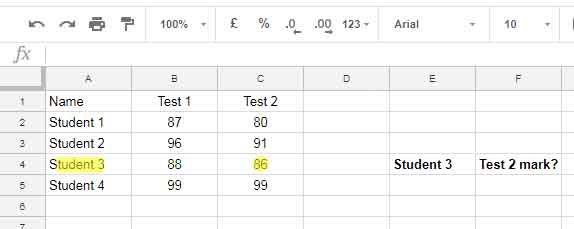

Sample dataset of student names and test scores demonstrating VLOOKUP in Google Sheets

Explanation:

"Student 3" → search key
A2:C5 → lookup range
3 → return value from the third column
FALSE → exact match

Result:

What VLOOKUP Does

VLOOKUP searches vertically down the first column of a range and returns a value from another column in the same row.

Exact Match vs Approximate Match

Exact Match (Recommended)

=VLOOKUP("Apple", A2:B10, 2, FALSE)

Returns an exact match only.

If no match is found, the formula returns #N/A.

Approximate Match

=VLOOKUP(75, A2:B10, 2, TRUE)

Returns the closest match less than or equal to the search key.

Use this only when the first column is sorted in ascending order.

Search Multiple Values Using VLOOKUP

You can search for multiple values at once using ARRAYFORMULA.

=ARRAYFORMULA(VLOOKUP(D2:D3, A2:B5, 2, FALSE))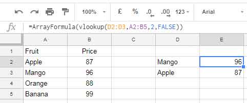

VLOOKUP formula with multiple search keys using ARRAYFORMULA in Google Sheets

You can also hardcode search keys:

=ARRAYFORMULA(VLOOKUP({"Mango"; "Apple"}, A2:B10, 2, FALSE))

Return an Entire Row

Use an array of column indexes to return multiple columns.

=ARRAYFORMULA(VLOOKUP("Student 2", A2:D5, {1, 2, 3, 4}, FALSE))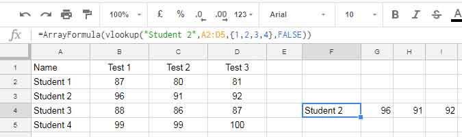

Returning a full row using VLOOKUP and ARRAYFORMULA in Google Sheets

Dynamic version:

=ARRAYFORMULA(
  VLOOKUP(
    "Student 2",
    A2:D5,
    SEQUENCE(1, COLUMNS(A2:D5)),
    FALSE
  )
)

This automatically adjusts when columns are added or removed.

Dynamic Column Index in VLOOKUP

Instead of hardcoding the column index, make it dynamic using COLUMNS().

=VLOOKUP("Student 2", A2:D5, COLUMNS(A2:D2), FALSE)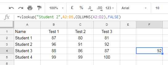

Dynamic VLOOKUP using the COLUMNS function to automatically adjust the column index

Benefits:

more flexible formulas,
safer when inserting columns,
easier maintenance.

Reverse (Leftward) VLOOKUP

VLOOKUP normally searches only from left to right.

You can reverse the lookup direction using array literals.

=VLOOKUP("Student 3", {D2:D5, A2:C5}, 2, FALSE)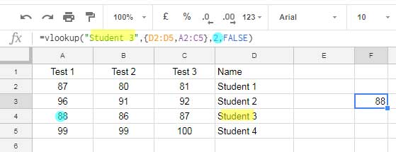

VLOOKUP workaround to search columns to the right in Google Sheets

This rearranges the lookup range virtually.

Case-Sensitive VLOOKUP

By default, VLOOKUP is not case-sensitive.

Example:

IL102B
IL102b

VLOOKUP treats both as the same.

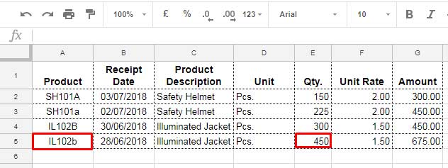
Case-sensitive lookup in Google Sheets using the QUERY function

One workaround is combining QUERY with VLOOKUP.

=VLOOKUP(
  "IL102b",
  QUERY(A2:G5, "SELECT * WHERE A = 'IL102b'"),
  5,
  FALSE
)

Related tutorial:
Case-Sensitive VLOOKUP in Google Sheets

VLOOKUP with Multiple Criteria

VLOOKUP supports multiple conditions by combining columns.

Example:

=ARRAYFORMULA(
  VLOOKUP(
    "CementZ",
    {A2:A7&B2:B7, C2:C7},
    2,
    FALSE
  )
)

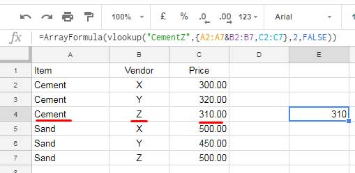
Combining item and vendor columns for a multi-condition VLOOKUP formula

This combines:

Product name
Vendor name

Wildcard Matching in VLOOKUP

VLOOKUP supports wildcard characters when FALSE is used.

Asterisk `*`

Matches multiple characters.

=VLOOKUP("Y*", A2:B6, 2, FALSE)

Question Mark `?`

Matches a single character.

Tilde `~`

Escapes wildcard characters.

Example:

~*

matches a literal asterisk.

Related tutorial:
Partial Match in VLOOKUP in Google Sheets

Named Ranges and Table References

Using Named Ranges

If A2:D5 is named sales:

=VLOOKUP("Student 3", sales, 4, FALSE)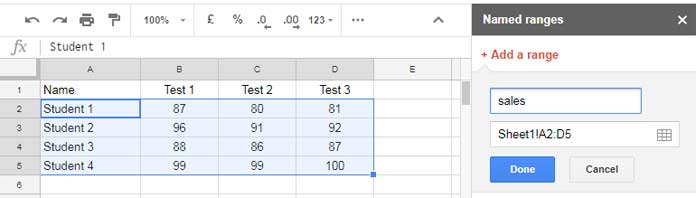

VLOOKUP using a named range to simplify formulas in Google Sheets

Named ranges improve formula readability.

Related tutorial:
Using Named Ranges in VLOOKUP

Using Table References

Google Sheets tables also support structured references.

=VLOOKUP("Apple", Table1, 2, FALSE)

This keeps formulas dynamic as tables expand.

VLOOKUP with IMPORTRANGE

You can combine VLOOKUP with IMPORTRANGE to search data from another spreadsheet.

Example:

=VLOOKUP(
  A2,
  IMPORTRANGE("spreadsheet_url", "Sheet1!A:D"),
  4,
  FALSE
)

Common VLOOKUP Errors

#N/A Error

Usually means:

no exact match found,
spelling mismatch,
extra spaces,
or incorrect lookup range.

Use IFNA to handle errors:

=IFNA(VLOOKUP(A2, B2:D10, 2, FALSE))

Incorrect Results

Often caused by:

using TRUE unintentionally,
unsorted data,
incorrect column index.

Related tutorial:
Common Errors in VLOOKUP in Google Sheets

VLOOKUP vs XLOOKUP

VLOOKUP is still useful, but XLOOKUP is more flexible.

XLOOKUP advantages:

searches left or right,
supports exact match by default,
returns arrays more easily,
handles missing values better,
can return a reference to the result cell.

Use VLOOKUP when:

performing simple vertical lookups,
returning a 2D array result.

Related tutorial:
VLOOKUP vs XLOOKUP in Google Sheets

When NOT to Use VLOOKUP

Consider alternatives when:

you need leftward lookups,
better error handling,
or more flexible matching.

Useful alternatives:

XLOOKUP
INDEX-MATCH
FILTER

Advanced VLOOKUP Tutorials

Multiple Matches and Duplicates

Cross-Sheet Lookups

Advanced Lookup Techniques

Dynamic Formula Techniques

Troubleshooting and Special Cases

Integrations and Combinations

Special VLOOKUP Techniques & Real-World Patterns

Aggregation & Combined Results

Date & Range-Based Lookups

Nested & Multi-Step Lookups

Layout & Structural Workarounds

Conclusion

VLOOKUP remains one of the most useful lookup functions in Google Sheets for beginners and advanced users alike.

Once you understand:

exact matches,
dynamic column indexes,
multiple criteria,
wildcard matching,
and cross-sheet lookups,

you can solve a wide range of spreadsheet problems efficiently.

If you regularly work with modern spreadsheets, also consider learning:

XLOOKUP,
FILTER,
and INDEX-MATCH

to build even more flexible formulas.

1 COMMENT

Bik M'Path June 22, 2019 At 12:33 am

The left-ward Vlookup, this was neat. Thanks for publishing this. All the best in saving the rest of us considerable time and grief, I know it helped me with Google Sheets.