When working with lookup functions in Google Sheets, a common need is to find the nearest match greater than or equal to a search key. While VLOOKUP is a classic choice, it doesn’t natively support this behavior. In this post, you’ll learn a simple VLOOKUP workaround to achieve this and also see how the newer XLOOKUP function makes this task easier.
VLOOKUP is still valuable because it can return multiple columns at once (a 2D array), a feature that XLOOKUP in Google Sheets doesn’t fully support yet.
Whether you’re replacing nested IF statements or handling grouped data, these techniques will simplify your Google Sheets formulas.
How VLOOKUP Handles Nearest Matches in a Sorted Range
By default, VLOOKUP in Google Sheets works on a sorted range and returns the nearest match less than or equal to the search key. For example:
=VLOOKUP(search_key, range, column_index, TRUE)- The
TRUE(or omitted) fourth parameter indicates an approximate match, where VLOOKUP finds the closest value less than or equal to your search key. - This works perfectly when your data is sorted ascending.
However, VLOOKUP does not support finding the nearest match greater than or equal to the search key. This limitation means you need a workaround or to switch to XLOOKUP.
Why XLOOKUP Is a Simpler Solution
Before diving into VLOOKUP hacks, it’s worth noting that Google Sheets now supports XLOOKUP, which easily handles nearest match greater than or equal to the search key.
Example:
=XLOOKUP(search_key, lookup_range, return_range, "Not Found", 1)- The last argument
1tells XLOOKUP to find the next larger or exact match. - This function is cleaner, simpler, and recommended.
Example Dataset: Age Groups and Population Percentage
Suppose you have age group data like this:
| Age Group Start | Age Group End | Percentage of Population (%) |
|---|---|---|
| 0 | 14 | 22.5 |
| 15 | 24 | 15.3 |
| 25 | 44 | 34.1 |
| 45 | 64 | 18.7 |
| 65 | 100 | 9.4 |
You want to input an age and return the corresponding population percentage.
Using SORTN with Logical Tests to Lookup Value Within a Range
With some knowledge of logical tests, you can identify the right row using a formula like this:
=SORTN(IF((A2:A <= E2) * (B2:B >= E2), C2:C), 1)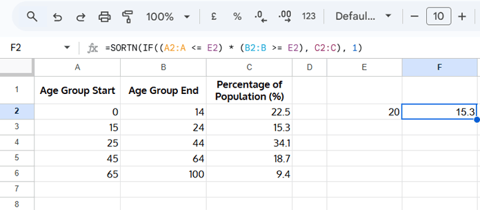
- Here,
E2contains the age to lookup. - This formula returns the percentage where the age falls within the start and end age group.
For example, if E2 = 20, it returns 15.3.
What If Your Age Group Data is Compressed?
Sometimes the data might look like this:
| Age Group | Percentage of Population (%) |
|---|---|
| 14 | 22.5 |
| 24 | 15.3 |
| 44 | 34.1 |
| 64 | 18.7 |
| 100 | 9.4 |
Here, the age group column only contains the end values of ranges.
XLOOKUP for Nearest Match Greater Than or Equal to Search Key
For the compressed table above, you can use this XLOOKUP formula if your search key is in E2:
=XLOOKUP(E2, A2:A, B2:B, "Not Found", 1)
- This will find an exact match or the next larger age group boundary.
- XLOOKUP natively supports nearest match greater than or equal to search key, making it ideal here.
VLOOKUP Workaround for Nearest Match Greater Than or Equal to Search Key
Since VLOOKUP cannot find the nearest greater than or equal match natively, here’s a neat hack:
How VLOOKUP Normally Works
- VLOOKUP with approximate match returns the nearest value less than or equal to the search key.
- We cannot change this default behavior.
The Workaround: Modify the Lookup Range Virtually
We virtually move the lookup column values down by one row by adding a zero at the top of the lookup column without changing the size of the return column.
How?
HSTACK(VSTACK(0, A2:A), B2:B)VSTACK(0, A2:A)adds a zero at the top of your lookup column and shifts all values down.HSTACK()pairs this modified column with your return columnB2:B.
Complete Formula Using VLOOKUP Workaround
=IFNA(
  VLOOKUP(E2, A2:B, 2, FALSE),
  VLOOKUP(E2, HSTACK(VSTACK(0, A2:A), B2:B), 2, TRUE)
)- The first
VLOOKUPattempts an exact match withFALSEas the last argument. - If no exact match is found (
IFNA), the secondVLOOKUPuses the modified range withTRUEfor approximate match to find the nearest greater than or equal value.
Which One Should You Use: VLOOKUP or XLOOKUP?
- XLOOKUP is simpler, more intuitive, and supports nearest greater or equal match natively.
- VLOOKUP can do it with the above workaround but is more complex.
- Use VLOOKUP if you need to search for multiple keys at once and return a 2D array, something that XLOOKUP currently does not support well. For example, the following formula uses keys in the range
E2:E3and returns values from columns B and C (a 2D array):
=ArrayFormula(IFNA(
  VLOOKUP(E2:E3, A2:C, {2, 3}, FALSE),
  VLOOKUP(E2:E3, HSTACK(VSTACK(0, A2:A), B2:C), {2, 3}, TRUE)
))
Additional Resources
- How to Lookup Latest Dates in Google Sheets
- Retrieve the Earliest or Latest Entry Per Category in Google Sheets
- Combine Rows and Keep Latest Values in Google Sheets
- Highlight the Latest Value Change Rows in Google Sheets
- How to Highlight the Latest N Values in Google Sheets
- Get the Latest Non-Blank Value by Date in Google Sheets
- Merge Duplicate Rows and Keep Latest Values in Excel


Please explain the
if(,,). How does it work?Hi, Rudy,
For learning the IF function, please check my Functions Guide.
If you use IF omitting arguments, for example,
if(,,), it will return a null (blank) value.Why don’t you use
""for the blank cell?Hi, Rudy,
You can use that also for the said purpose in Vlookup.
But it won’t serve the purpose in ALL functions, especially in DATABASE functions where you should use the IF.