When you need to send pre-filled Google Forms with varying answers to responders, Google Sheets becomes an invaluable tool.
Customizing pre-filled links within Google Sheets is achieved by utilizing two functions: SUBSTITUTE and ENCODEURL. Additionally, the MAP Lambda function can be employed to generate multiple pre-filled links simultaneously.
When Does Pre-filled Google Forms Come in Handy?
Consider a scenario where you maintain a customer database, and some customer data is missing.
By filling the Google Forms with available data and sending them to customers, you enable them to complete the missing information and update existing details.
This approach offers two key benefits. First, customers are spared from filling out all the data, saving them time. Second, they can adhere to a predefined format while providing the information.
Now, let’s explore a step-by-step guide on how to automatically pre-fill Google Forms from Google Sheets.
Copy the Pre-filled Link from a Google Forms Form
Let’s initiate the process by starting with Google Forms and then transitioning to Google Sheets.
For illustrative purposes, let’s consider a Google Forms form with the following questions and question types:
| Question | Question Type |
| Name | Short answer |
| Date of Birth | Date |
| Gender | Short answer |
| Email Address | Short answer |
| Website URL | Short answer |
Note: If you want to learn about all question types in a Google Docs Form, please check out this guide: How to Set Up Google Docs Forms – A Comprehensive Guide.
The initial step involves populating the relevant fields with mockup answers. This is essential to obtain a pre-filled link that we will later edit in Google Sheets.
Open the form, click on the three vertical dots menu in the top right, and select “Get pre-filled link.”
Fill out the form with mockup answers. It will resemble the following:
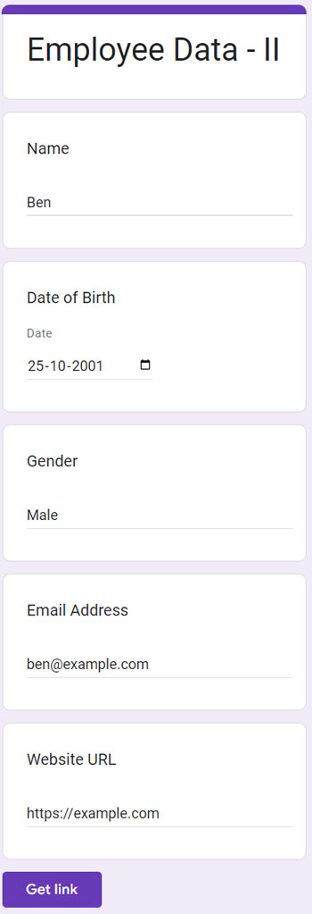
Click on the “Get Link” button at the bottom of the form to reveal the “Copy Link” button. Click “Copy Link.”
The subsequent steps for automatically pre-filling a Google Forms form will be carried out within Google Sheets.
Arranging Data in Google Sheets for Pre-fill Google Forms Dynamically
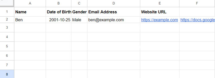
In a blank Google Sheets spreadsheet, paste the copied link into cell F2.
In cells A1 to E1, input the questions as follows, which are taken from the form itself:
- “Name” in A1
- “Date of Birth” in B1
- “Gender” in C1
- “Email Address” in D1
- “Website URL” in E1
Directly below, copy and paste the relevant answers from the link in cell F2. These answers can be easily identified in the URL as they are followed by unique identifiers.
Example URL:
https://docs.google.com/forms/d/e/1FAIpQLSdODZyp4VArdGQaR7B3b_OoENyJiSTaRWC71SkhSiUQSb-COQ/viewform?usp=pp_url&entry.1724134270=Ben&entry.2056058142=2001-10-25&entry.640660802=Male&entry.1368777253=[email protected]&entry.1046411540=https://example.comIt should look like as follows.
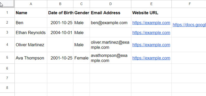
Now, input data in cell range A3:E that you want to automatically pre-fill in Google Forms. Please refer to the screenshot below:
Key Points
We cannot pre-fill answers for question types such as multiple choices, checkboxes, and drop-downs. I recommend avoiding the use of these question types in Sheets to ensure they remain in their default state in the form.
For Date question answers, they must be entered as they appear in the link, which is in the YYYY-MM-DD format. To ensure accurate entry, consider applying Format > Plain Text to the range B3:B5, and then enter the date in the specified format, as demonstrated in the example.
Formula to Automatically Pre-fill a Google Forms Form from Google Sheets
To automatically replace the mockup answers in the link in cell F2 (which we copy-pasted in A2:E2) with the original answers in A3:E3, we’ll utilize the SUBSTITUTE function in a nested form. This formula should be applied in cell F3.
The SUBSTITUTE function replaces existing text with a new one.
Syntax of the SUBSTITUTE Function:
SUBSTITUTE(text_to_search, search_for, replace_with, [occurrence_number])In this context, the text_to_search is the link in cell F2. Now, let’s discuss search_for and replace_with.
In the first SUBSTITUTE, search_for is the text in A2, and replace_with is the text in A3. We should use it as follows:
=SUBSTITUTE($F$2, "="&$A$2, "="&ENCODEURL(A3))You might wonder, why not use =SUBSTITUTE($F$2, $A$2, A3) directly?
In URLs, spaces and some other characters are not allowed, which can lead to issues in parsing and processing. The ENCODEURL function addresses those issues.
If you inspect the link in cell F2, you’ll notice that each answer starts with an = sign. Utilizing it with search_for and replace_with ensures that the SUBSTITUTE function replaces only the answers, avoiding errors, especially when dealing with short answers like “F” for females or “M” for Males.
Note: The letter ‘P’ is an exception to this, as the letter ‘p’ starts with an = sign other than as an answer (e.g., =pp_url). Therefore, you must avoid replacing the short answer “P” (if any) using SUBSTITUTE.
Now, we should nest this formula within additional SUBSTITUTE functions to handle B2 and B3, C2 and C3, and so on. Here’s the nested SUBSTITUTE formula:
=SUBSTITUTE(
   SUBSTITUTE(
      SUBSTITUTE(
         SUBSTITUTE(
            SUBSTITUTE($F$2, "=" & $A$2, "=" & ENCODEURL(A3)),
         "=" & $B$2, "=" & ENCODEURL(B3)),
      "=" & $C$2, "=" & ENCODEURL(C3)),
   "=" & $D$2, "=" & ENCODEURL(D3)),
"=" & $E$2, "=" & ENCODEURL(E3))
Copy this formula down for further application.
Clicking on the links in cells F2, F3, F4, and F5 will take you to Google Forms with various pre-filled answers.
How Can We Convert This Into an Array Formula?
Understanding what happens when you drag down the formula in cell F3 is crucial to converting it into an array formula.
When you drag the formula that facilitates autofill for Google Forms in Google Sheets, the cell ranges A3, B3, C3, D3, and E3 increment as they are relative references in the formula. Other cell references are absolute.
This relative referencing ensures that the formula substitutes the mockup data with data from the current row.
To achieve this more efficiently, we can use the MAP function to refer to arrays A3:A5, B3:B5, C3:C5, D3:D5, and E3:E5, and iterate over each value in this array.
First, empty the range F3:F5, and then insert the following array formula into cell F3:
=MAP(
   A3:A5, B3:B5, C3:C5, D3:D5, E3:E5,
   LAMBDA(a, b, c, d, e,
     SUBSTITUTE(
        SUBSTITUTE(
           SUBSTITUTE(
               SUBSTITUTE(
                   SUBSTITUTE(F2, "="&A2, "="&ENCODEURL(a)),
               "="&B2, "="&ENCODEURL(b)),
           "="&C2, "="&ENCODEURL(c)),
        "="&D2, "="&ENCODEURL(d)),
     "="&E2, "="&ENCODEURL(e))
   )
)
After entering the array formula in cell F3, no additional dragging is required. The formula, being an array formula, will automatically extend its application to the entire range F3:F5 without the need for manual dragging.
Formula Explanation
The formula uses the MAP function along with the LAMBDA function to create an array formula. Here’s a brief explanation:
The MAP function iterates over arrays A3:A5, B3:B5, C3:C5, D3:D5, and E3:E5, applying a lambda function (anonymous function) to each corresponding set of values. The lambda function, expressed with LAMBDA(a, b, c, d, e, ...), uses the SUBSTITUTE function to replace mockup data in the link in cell F2 with actual data from the current row.
In simpler terms, this array formula dynamically replaces values in F2 based on the corresponding values in the specified arrays for each row.


