With the help of EOMONTH, UNIQUE, and SUMIFS functions in Excel, you can efficiently sum values in a range by month and category.
In the summary report, the first column will contain the unique categories, while the first row will span across months in a year, typically labeled from January to December.
Each cell in the table will contain the corresponding values representing the expenditure or allocation amount for each category during each month.
There are two approaches: One is the regular approach, which involves using helper columns and drag-down formulas. The other is an advanced approach using dynamic array formulas. The latter approach is suitable for users of Excel for Microsoft 365.
Sum Values by Month and Category in Excel: Regular Approach
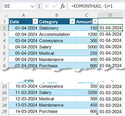
The sample data consists of Date, Category, and Amount in cell range A1:C29, where A1:C1 contains the labels. Here are the step-by-step instructions:
Step 1: Helper Column to Convert Dates to Beginning of the Month Dates
In this regular approach, we require a helper column to sum values in a range by month and category. Let’s prepare that first.
In cell D2, enter =EOMONTH(A2, -1)+1, which will return the beginning of the month date of the date in cell A2.
Click and drag the fill handle at the bottom right corner of cell D2 until your last row in the range, here D29.
Step 2: Preparing the First Row and First Column for the Month and Category Wise Summary Report
Key in the following Excel formula in cell F2 to return unique categories in the range B2:B29:
=UNIQUE(B2:B29)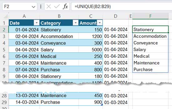
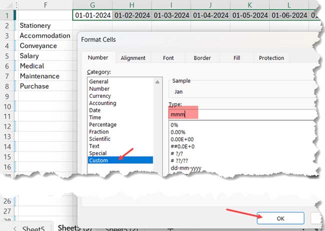
Enter the beginning of the month dates 1/1/2024 and 1/2/2024 in cells G1 and H1 respectively.
Select G1:H1 and drag the fill handle across until R1.
Select G1:R1, right-click to open the context menu, and click on “Format Cells.”
In the Format Cells dialog box, click Custom under the Number tab and enter “mmm” under the type field.
Click OK.
We are now set to use the SUMIFS formula to sum by month and category.
Step 3: SUMIFS Formula to Sum by Month and Category in Excel
In cell G2, enter the following SUMIFS formula:
=SUMIFS($C$2:$C$29, $B$2:$B$29, $F2, $D$2:$D$29, G$1)This follows the syntax SUMIFS(sum_range, criteria_range1, criteria1, criteria_range2, criteria2)
Where:
sum_range: $C$2:$C$29criteria_range1: $B$2:$B$29criteria1: $F2criteria_range2: $D$2:$D$29criteria2: G$1
Click the fill handle of cell G2 down until cell G8.
Select G2:G8, click, and drag the fill handle at the bottom right corner of cell G8 across to R8.
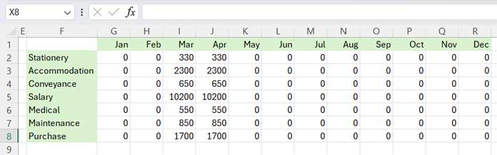
This way, we use SUMIFS with UNIQUE and EOMONTH to sum values by month and category in Excel.
Sum Values by Month and Category in Excel: Dynamic Array Formula Approach
One of the advantages of this formula is that it doesn’t require the helper column D, which represents the beginning of the month.
In three steps, you can create month and category-wise summaries using this dynamic formula approach in Excel for Microsoft 365:
- Enter
=UNIQUE(B2:B29)in cell F2 to generate the list of unique categories. - Enter
=EDATE(DATE(2024, 1, 1), SEQUENCE(1, 12, 0))in cell G1 to generate the beginning of the month dates (date values) from January to December 2024 in G1:R1. If you want a different year, replace “2024” in the formula with the desired year.
You may select G1:R1, right-click to open the context menu, and click on “Format Cells.” Then, click on “Custom” and enter “mmm” in the type field. Please scroll up and refer to the relevant screenshot. - Now, insert the following dynamic array formula in cell G2 to generate the month and category-wise summary for all the months and categories.
=LET(
   dt, A2:A29,
   category, B2:B29,
   amount, C2:C29,
   u_category, F2:F8,
   header, G1:R1,
   DROP(
      REDUCE(0, header, LAMBDA(a, v, HSTACK(a,
         MAP(u_category, LAMBDA(cat,
            SUMPRODUCT((category=cat)*
            (MAP(dt, LAMBDA(dt, EOMONTH(dt, -1)+1))=v)*
            amount)
         ))
      ))), 0, 1
   )
)
How Do I Use this Formula in a Completely Different Range in my Excel Spreadsheet?
Please see the highlighted range references in the formula above. You need to make changes to those references.
- A2:A29: Replace it with the date range in your spreadsheet.
- B2:B29: Replace it with the category range in your spreadsheet.
- C2:C29: Replace it with the amount range in your spreadsheet.
- F2:F8: Replace it with the unique category range returned by the UNIQUE formula.
- G1:R1: Replace it with the range of the beginning of month dates returned by the EDATE formula.
Resources
Here are some related resources for Excel.


