To sum by week number, we’ll utilize the WEEKNUM, UNIQUE, and SUMIF functions in Excel using the traditional approach.
If you prefer a dynamic array formula to accomplish this task, then SUMIF won’t suffice. Instead, we’ll replace it with SUMPRODUCT and utilize the MAP lambda function to generate an array result. The dynamic array formula avoids helper columns and creates a week number summary that spills down.
We’ll examine both options.
Setting Up the Sample Data
We need at least two columns of data: one containing dates and the other containing values to sum.
Consider the following data in cell range A1:B10 in an Excel spreadsheet:
| DATE | VALUE |
| 01-04-2024 | 5 |
| 05-04-2024 | 4 |
| 10-04-2024 | 5 |
| 12-04-2024 | 6 |
| 13-04-2024 | 5 |
| 22-04-2024 | 5 |
| 25-04-2024 | 4 |
| 26-04-2024 | 5 |
| 27-04-2024 | 4 |
Follow the steps below to sum by week numbers in Excel.
Sum by Week in Excel: Traditional SUMIF and WEEKNUM Approach
The formula is a SUMIF, but we will use the WEEKNUM and UNIQUE functions to extract week numbers and make them unique.
Syntax: SUMIF(range, criteria, [sum_range])
range:
We need to extract the week numbers from the dates in A2:A10. Enter the following formula in cell D2:
=WEEKNUM(A2)Click and drag the bottom right fill handle (which turns into a plus sign) in cell D2 down to cell D10.
criteria:
In cell E2, enter the following UNIQUE formula to return an array containing unique week numbers:
=UNIQUE(D2:D10)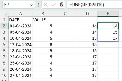
sum_range:
The sum_range, which we will specify inside the SUMIF formula, is B2:B10.
Sum by Week Number Formula:
In cell F2, enter the following formula and drag the fill handle until F4:
=SUMIF($D$2:$D$10, E2, $B$2:$B$10)$D$2:$D$10 represents the range, E2 is the criteria, and $B$2:$B$10 is the sum_range.
Note: The formula considers Sunday to Saturday weeks for week number extraction. If your week starts on Monday and ends on Sunday, use =WEEKNUM(A2, 2) instead of =WEEKNUM(A2).
Sum by Week Using a Dynamic Array Formula in Excel
Disclaimer:
I tested the following formula in Excel in Microsoft 365. It will not function in Excel versions that lack dynamic array formula functionality.
Formula:
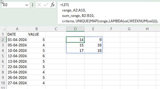
=LET(
   range, A2:A10,
   sum_range, B2:B10,
   criteria, UNIQUE(MAP(range,LAMBDA(val,WEEKNUM(val)))),
   HSTACK(
      criteria,
      MAP(criteria, LAMBDA(val,
         SUMPRODUCT(
            (MAP(range, LAMBDA(val, WEEKNUM(val)))=val)*sum_range
         )
      ))
   )
)
How do I use this formula?
Input this formula into cell D2. It will return the sum by week without needing to be dragged down.
When using this Excel dynamic array formula with your table, replace A2:A10 with the date range (range) and B2:B10 with the sum range.
This formula takes care of everything on its own!
How Can I Specify a Different Week Start and End?
In the dynamic array formula for sum by week, you can see the use of WEEKNUM(val) twice. It uses week number type 1, which corresponds to Sunday to Saturday.
To specify Monday to Sunday, replace them with WEEKNUM(val, 2). The “2” in this WEEKNUM function is called return_type in Excel.
For the return_types, please refer to this table:
| Week | return_type |
| Sun-Sat | 1 or omitted |
| Mon-Sun | 2 |
| Mon-Sun | 11 |
| Tue-Mon | 12 |
| Wed-Tue | 13 |
| Thu-Wed | 14 |
| Fri-Thu | 15 |
| Sat-Fri | 16 |
| Sun-Sat | 17 |
| Mon – Sun | 21 |
In return_types 1, 2, and 11 to 17, the week containing January 1st is considered as week 1. In return_type 21, the week containing the 1st Thursday of the year is numbered as week 1.


