Do you know how to create sequential dates in equally merged cells across a row or down a column in Google Sheets?

Sometimes we may have equally merged cells, for example, a date in the header row merged across two cells and below two labels representing two activities on that date. And we might want a sequence of dates in equally sized merged cells in the header row.

The issue with merged cells is that, although the formula inserts date into all cells regardless of whether they are merged or unmerged, only the value in the first cell of the merged cells is displayed. So, you will see dates skipping. The underlying values in the hidden cells are still there and can be accessed if you unmerge the cells.

In this tutorial, you can learn how to use a formula in Google Sheets to insert sequential dates into equally sized merged cells. The underlying value in the hidden cells won’t be dates or numbers, so it may not affect any calculations you want to perform.

Sequential Dates in Equally Merged Cells Across a Row

In the following example, I want sequential dates in the range B1:O1, which comprises 14 cells. Each pair of cells is merged, so there should be seven dates.

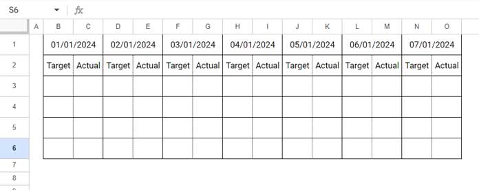
As a side note, you can find the number of cells across a range using the COLUMNS function, like so: =COLUMNS(B1:O1).

Here is the formula to use in cell B1, provided B1:O1 is empty beforehand:

=ArrayFormula(LET(
     start, DATE(2024, 1, 1), 
     m_cells, 2, 
     n, 7, 
     seq, SEQUENCE(1, n*m_cells, m_cells)/m_cells, 
     IF(MOD(seq, 1)=0, start+seq-1, " ")
))

You may select the result range and apply Format > Number > Date to format the date values as dates.

In this formula:

• start: DATE(2024, 1, 1) – the starting date in the sequence in the syntax DATE(year, month, day).
• m_cells: 2 – the number of cells merged in each pair across the row.
• n: 7 – the total number of dates you want in the sequence.

Assume you want 30 sequential dates in three equally merged cells across a row.

Replace 2 (m_cells) with 3 and 7 (n) with 30.

Sequential Dates in Equally Merged Cells in a Column

I want sequential dates in merged cells in a column. Please refer to the image below.

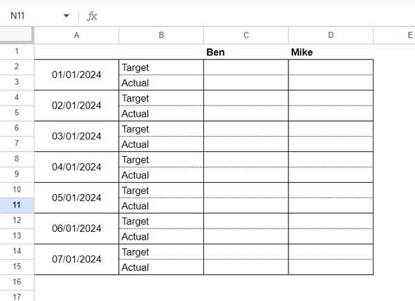
I want seven sequential dates in cells A2:A15, which comprise 14 cells, with every two cells merged. (You can use the ROWS function to find the number of cells in a column, like this: =ROWS(A2:A15))

You need to insert this formula into cell A2 after clearing any contents in A2:A15:

=ArrayFormula(LET(
     start, DATE(2024, 1, 1), 
     m_cells, 2, 
     n, 7, 
     seq, SEQUENCE(n*m_cells, 1, m_cells)/m_cells, 
     IF(MOD(seq, 1)=0, start+seq-1, " ")
))

Similar to the formula for a row, you should format the result range to date by selecting A2:A15 and clicking Format > Number > Date.

In this formula:

• start: DATE(2024, 1, 1) – represents the starting date in the sequence using the syntax DATE(year, month, day).
• m_cells: 2 – indicates the number of cells merged in each pair in the column.
• n: 7 – signifies the number of dates you want in the sequence.

Will the Formula Work if the Range is Not Merged?

Yes, the formula will return dates across the row or down the column, depending on the formula in use.

It will include blank cells between dates based on the value you specified in the m_cells parameter.

If you specify 2, it will return one blank cell; for 3, two blank cells, and so on. Please note that the blank cells contain a space character, not purely blank.

Formula Breakdown

I followed the logic below to create sequential dates in equally merged cells in Google Sheets.

Let’s consider the function for the row. Here is the breakdown of the formula:

=SEQUENCE(1, 7)

The above SEQUENCE function will return the numbers 1 to 7 in a row.

The Syntax is:

=SEQUENCE(rows, [columns], [start], [step])

Assuming you have uniquely merged cells in the range B1:O1, and each merged area contains two cells. Therefore, there will be 14 merged areas for 7 sequential dates.

What you should do here is, generate 14 sequential numbers, and the sequence should start from 2, which is the number of merged cells in each merged area.

=SEQUENCE(1, 7*2, 2)

Now divide these by 2.

=ArrayFormula(SEQUENCE(1, 7*2, 2)/2)

The formula requires the ARRAYFORMULA function as we performed the division operation in an array.

The formula will return integers at the start of every merged cell and decimals in the ‘hidden’ cells.

Now, what we should do is to return a space wherever the SEQUENCE formula returns decimals. We can use a logical test for that.

Let’s call the above formula ‘seq’, and here is that logical test.

IF(MOD(seq, 1)=0, start+seq-1, " ")

The IF and MOD combo checks if the sequence number (seq) is divisible by 1 without any remainder, meaning it’s a whole number.

This formula generates sequential numbers starting from a specified “start” value, only in cells where the sequence is a whole number. The start value is the start date of the sequence.

I’ve utilized the LET function to define names within the formula.

Resources

• Sequence Numbering in Merged Cells In Google Sheets
• How to Fill Merged Cells Down or to the Right in Google Sheets
• How to Populate Sequential Dates Excluding Weekends in Google Sheets
• Auto-Fill Sequential Dates When Value Entered in Next Column in Google Sheets
• Adding N Blank Rows to SEQUENCE Results in Google Sheets