The ARRAYFORMULA function in Google Sheets lets you apply a formula to an entire range of cells and return multiple results automatically. Instead of copying the same formula down a column or across a row, you can write a single array formula that expands the results to multiple cells.

Unlike Microsoft Excel, Google Sheets originally did not support automatic dynamic array spilling for most formulas. The ARRAYFORMULA function fills this gap by allowing formulas to process ranges and return multiple results at once.

In simple terms, ARRAYFORMULA enables one formula to replace many individual formulas in a worksheet.

Although some functions such as INDEX can also return arrays, the ARRAYFORMULA function is the primary and most efficient way to create array formulas in Google Sheets. In most cases, wrapping a formula with ARRAYFORMULA is the easiest way to apply calculations to an entire column or range.

In this tutorial, you will learn:

• The syntax of the ARRAYFORMULA function
• Simple and practical ARRAYFORMULA examples
• When to use ARRAYFORMULA and when not to
• How ARRAYFORMULA works with functions like VLOOKUP, XLOOKUP, COUNTIF, and SUMIF

ARRAYFORMULA Function: Syntax and Arguments

Syntax of the ARRAYFORMULA Function in Google Sheets

ARRAYFORMULA(array_formula)

The ARRAYFORMULA function has only one argument: array_formula.

ARRAYFORMULA Function Argument

array_formula – The formula or expression that you want to apply to a range of cells and return multiple results.

Notes and Examples

The array_formula argument can contain different types of expressions. The most common ones are explained below.

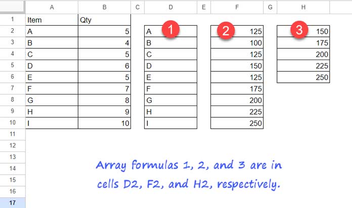
1. Using a Cell Range

The argument can simply be a range of cells.

Example:

=ARRAYFORMULA(A2:A10)

This formula returns the values in the range A2:A10 as an array result.

2. Using a Mathematical Expression

You can perform calculations on an entire range of values.

Example:

=ARRAYFORMULA(B2:B10*25)

This formula multiplies each value in B2:B10 by 25 and returns the results in multiple rows.

3. Using a Function That Returns Multiple Results

The ARRAYFORMULA function can also wrap functions that return multiple values.

Example:

=ARRAYFORMULA(FILTER(B2:B10, B2:B10>5)*25)

This formula first filters the values in B2:B10 that are greater than 5, and then multiplies each returned value by 25.

ARRAYFORMULA Examples in Google Sheets

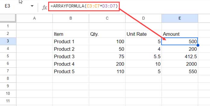
The following example shows how to use the ARRAYFORMULA function in Google Sheets to calculate values for multiple rows using a single formula.

Assume that column C contains quantities and column D contains unit rates. To calculate the amount for each product listed in B3:B7, enter the following array formula in cell E3:

=ARRAYFORMULA(C3:C7*D3:D7)

This formula multiplies each value in C3:C7 by the corresponding value in D3:D7 and returns the results in multiple rows automatically.

Without ARRAYFORMULA, you would normally enter the formula:

=C3*D3

in cell E3 and then copy or fill the formula down to the remaining rows.

How to Enter the ARRAYFORMULA Function

There are two ways to enter the ARRAYFORMULA function in Google Sheets.

1. Manually

Type:

=ARRAYFORMULA(

Then enter the formula you want to expand and press Enter.

2. Using the Keyboard Shortcut

Type the formula normally (starting with =), then press:

• Ctrl + Shift + Enter (Windows)
• ⌘ + Shift + Enter (Mac)

Google Sheets will automatically wrap your formula in ARRAYFORMULA.

Filling a Non-Array Formula Down

If you do not use ARRAYFORMULA, you must copy the formula (one that doesn’t use ranges) to the rows below. You can do this in several ways:

Copy and paste

1. Press Ctrl + C (Windows) or ⌘ + C (Mac) in cell E3.
2. Select cells E4:E7.
3. Press Ctrl + V (Windows) or ⌘ + V (Mac).

Auto-fill with a shortcut

1. Select E3:E7.
2. Press Ctrl + Enter (Windows) or ⌘ + Enter (Mac).

Use the fill handle

Drag the fill handle (the small square/circle in the bottom-right corner of the selected cell) downward.

More Basic ARRAYFORMULA Examples

Here are a few more practical examples of the ARRAYFORMULA function in Google Sheets.

Extract the first two characters from a range of text

=ARRAYFORMULA(LEFT(A2:A10, 2))

Returns the first two characters from each value in A2:A10.

Convert dates to month-end dates

=ARRAYFORMULA(TO_DATE(IFERROR(EOMONTH(DATEVALUE(B1:B1000), 0))))

Converts the dates in B1:B1000 to their corresponding month-end dates.

Combine first and last names

=ARRAYFORMULA(A1:A100&" "&B1:B100)

Joins the values in A1:A100 and B1:B100 with a space between them.

5 Things to Keep in Mind When Using ARRAYFORMULA in Google Sheets

Understanding how and when to use the ARRAYFORMULA function in Google Sheets is important for avoiding errors and maintaining good spreadsheet performance.

The following five points will help you use ARRAYFORMULA more effectively and troubleshoot common issues.

Performance-Related Tips

1. Ensure there are enough blank cells for the array result

An array formula must have enough empty cells to expand its results. If the destination cells already contain data, the formula will return a #REF! error.

2. Place formulas using open ranges in the first row or column

When using open ranges such as A2:A, place the formula in the first row (for vertical ranges) or the first column (for horizontal ranges) of the range’s starting point. This ensures the array formula expands correctly.

For example, the following formula entered in cell C3 may return the error:

=ARRAYFORMULA(ROW(A2:A))

Error message:

Result was not expanded automatically, please insert more rows.

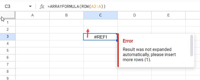
Entering this formula in row 3 or any lower row can also cause Google Sheets to add many blank rows at the bottom of the sheet, which may negatively affect performance.

Functionality-Related Tips

3. ARRAYFORMULA may expand intermediate results instead of the final function

Not all uses of ARRAYFORMULA are meant to return array outputs directly. In some cases, the function expands the result of another function inside the formula.

Example:

=ARRAYFORMULA(COUNTIF(YEAR(B1:B), 2023))

This formula counts the number of dates in B1:B that belong to the year 2023. Here, ARRAYFORMULA expands the YEAR function, allowing COUNTIF to evaluate the results.

Another example:

=ARRAYFORMULA(AND(C2:C5>5))

In this formula, ARRAYFORMULA expands the expression C2:C5>5, not the AND function.

4. Some functions do not work well with ARRAYFORMULA

Certain functions in Google Sheets cannot expand properly when wrapped in ARRAYFORMULA.

A simple rule of thumb:

If a non-criteria-based function accepts a range and returns a single result, it usually cannot be expanded with ARRAYFORMULA.

Examples include:

• SUM
• MAX
• ISDATE
• AND
• OR

Example:

=AND(C2:C6)

This formula returns TRUE only if all values in C2:C6 are TRUE; otherwise it returns FALSE. Since it produces a single result, ARRAYFORMULA cannot expand it.

In contrast, many criteria-based functions can expand because they evaluate each value individually.

Examples include:

• COUNTIF
• SUMIF
• VLOOKUP
• XLOOKUP
• IF

However, behavior may vary when multiple criteria ranges are used. For example:

• COUNTIFS can return array results.
• SUMIFS typically does not expand as an array.

5. Some functions already return arrays automatically

Certain functions in Google Sheets automatically spill results into neighboring cells, so ARRAYFORMULA is not required.

Examples include:

• SEQUENCE
• INDEX
• QUERY
• FILTER
• SORT
• IMPORTRANGE
• VSTACK
• HSTACK
• SWITCH

These functions are designed to return multiple values without needing ARRAYFORMULA.

Related: Google Sheets Function Guide.

Benefits of Using the ARRAYFORMULA Function in Google Sheets

The ARRAYFORMULA function in Google Sheets offers several advantages when working with large datasets or repetitive calculations. Instead of copying formulas across many rows or columns, you can use a single array formula to handle the entire range.

Here are the main benefits of using ARRAYFORMULA.

1. Improved Spreadsheet Performance

An array formula can replace hundreds or even thousands of individual formulas in a sheet. Instead of calculating each row separately, Google Sheets evaluates the entire range at once, which can help improve overall spreadsheet performance.

2. Easier Formula Maintenance

When you use ARRAYFORMULA, you only need to edit one formula in a single cell. Any modification automatically applies to the entire result range, making updates faster and easier.

3. Reduced Risk of Formula Errors

In traditional formulas, adding or deleting rows can sometimes leave cells without formulas or break the calculation pattern. With ARRAYFORMULA, the formula automatically expands to new rows, helping prevent missing or inconsistent formulas.

4. Faster Data Cleanup

Array formulas also make it easier to clean up a spreadsheet. Instead of deleting formulas in hundreds of cells, you can remove them by simply deleting the single array formula cell that generates the results.

How to Use ARRAYFORMULA with VLOOKUP, XLOOKUP, COUNTIF, and SUMIF in Google Sheets

The ARRAYFORMULA function in Google Sheets can also be combined with lookup and aggregation functions to process multiple criteria at once.

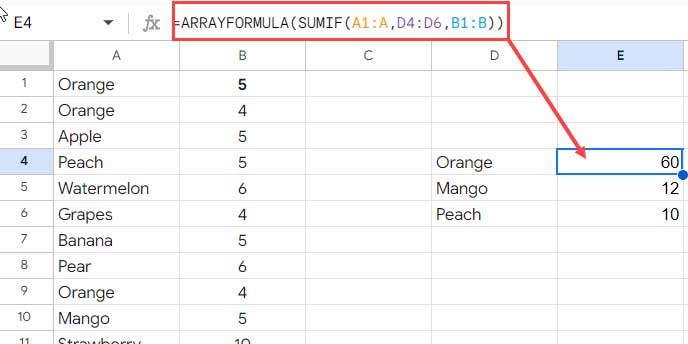
Assume we have a dataset of 10 fruits and their native origins in the range A1:B11, where:

• A2:A11 contains fruit names
• B2:B11 contains their native origins
• A1 and B1 contain the column headers

The search values are “Strawberry” and “Mango” in cells D2:D3.

Using ARRAYFORMULA with VLOOKUP

To return the native origins of the fruits listed in D2:D3, you can use the following ARRAYFORMULA + VLOOKUP formula:

=ARRAYFORMULA(VLOOKUP(D2:D3, A2:B11, 2, FALSE))

VLOOKUP Syntax

VLOOKUP(search_key, range, index, [is_sorted])

This formula searches the fruit names in D2:D3 within A2:A11 and returns the corresponding native origins from column B.

Using ARRAYFORMULA with XLOOKUP

You can achieve the same result using XLOOKUP, which provides a more flexible lookup method.

=ARRAYFORMULA(XLOOKUP(D2:D3, A2:A11, B2:B11))

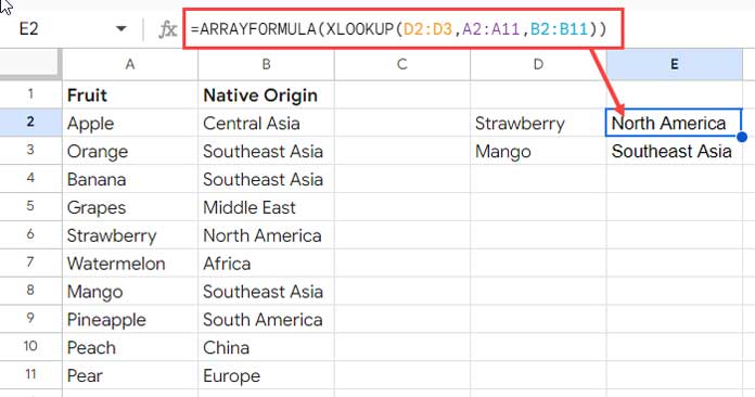
XLOOKUP Syntax

XLOOKUP(search_key, lookup_range, result_range, [missing_value], [match_mode], [search_mode])

This formula returns the native origins of Strawberry and Mango from the dataset.

Related: VLOOKUP and XLOOKUP: Key Differences in Google Sheets.

Using ARRAYFORMULA with COUNTIF

Suppose you want to count how many times “North America” and “Southeast Asia” appear in the range B2:B11.

If the criteria are in D2:D3, you can use:

=ARRAYFORMULA(COUNTIF(B2:B11, D2:D3))

COUNTIF Syntax

COUNTIF(range, criterion)

This formula returns the number of matches for each criterion in D2:D3.

Using ARRAYFORMULA with SUMIF

You can also combine ARRAYFORMULA with SUMIF to calculate totals based on multiple criteria.

For example:

=ARRAYFORMULA(SUMIF(A1:A, D4:D6, B1:B))

This formula returns the sum of values in column B for each matching value in column A, based on the criteria listed in D4:D6.

What LAMBDA Can Do That ARRAYFORMULA Can’t

This is an additional tip.

As explained earlier, the ARRAYFORMULA function in Google Sheets cannot expand every type of formula. Some functions always return a single result, even when they are used with a range of values.

For example, the following MIN function returns only one value for the row:

=MIN(B2:E2)

If you try to expand this formula with ARRAYFORMULA, it will not return separate results for each row.

However, you can achieve this using LAMBDA helper functions such as BYROW.

Example:

=BYROW(B2:E5, LAMBDA(v, MIN(v)))

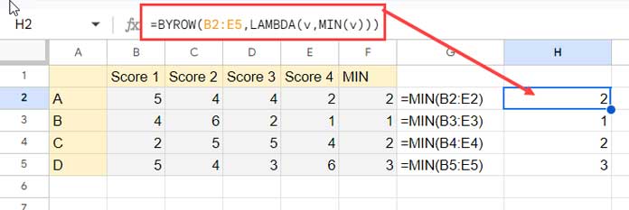
This formula applies the MIN function to each row in the range B2:E5 and returns the minimum value for every row. In other words, BYROW processes each row individually, which allows the formula to return multiple results.

Frequently Asked Questions About ARRAYFORMULA in Google Sheets

What does the ARRAYFORMULA function do in Google Sheets?

The ARRAYFORMULA function in Google Sheets allows you to apply a formula to an entire range of cells and return multiple results automatically. Instead of copying the same formula to each row or column, you can write one formula that expands the results across multiple cells.

When should I use ARRAYFORMULA in Google Sheets?

You should use ARRAYFORMULA when you want to apply the same calculation to multiple rows or columns. It is especially useful when working with large datasets because it allows you to replace many individual formulas with a single formula.

Why is my ARRAYFORMULA not expanding?

An ARRAYFORMULA may not expand if:

• There are existing values in the cells where the results should appear
• The formula does not support array expansion
• The formula is placed below the starting row of an open range

In such cases, Google Sheets may return a #REF! error or display a message indicating that the result could not be expanded.

Do all functions work with ARRAYFORMULA?

No. Some functions always return a single result, even when used with ranges. Examples include SUM, MAX, AND, and OR. These functions typically cannot expand with ARRAYFORMULA because they aggregate values into one result.

Do I always need ARRAYFORMULA in Google Sheets?

No. Some functions automatically return multiple results without requiring ARRAYFORMULA. Examples include FILTER, QUERY, SEQUENCE, SORT, and IMPORTRANGE. These functions already support dynamic array outputs.

Conclusion

Learning the ARRAYFORMULA function in Google Sheets is one of the first steps toward building efficient spreadsheets. Array formulas allow you to apply calculations to entire ranges using a single formula, which reduces repetition and improves maintainability.

Using ARRAYFORMULA effectively can:

• simplify large spreadsheets
• reduce the number of formulas in your sheet
• make updates and corrections easier

For better performance, keep only the necessary rows and columns in your worksheet, and be cautious when using open ranges. Proper use of ARRAYFORMULA can significantly improve both the speed and reliability of your spreadsheets.