The LEN function returns the length of a string, which is particularly useful in logical tests in Google Sheets. We can use this function mainly in two ways:
- With the IF function to evaluate whether a cell has a value or not.
- Within data validation to allow or reject strings of a particular length.
Before we delve into that, let’s examine the syntax of the LEN function in Google Sheets.
Syntax and Arguments
LEN(text)The function has only one argument, which is ‘text’. This is the string input for which the length will be returned.
However, it’s worth noting that the LEN function can also return the length of dates, numbers, or timestamps in a cell. Though usually, we may not need to find the length of such values.
Examples:
=LEN("APPLE") // returns 5
=LEN(123456789) // returns 9
In the following example, I’ve mixed data types in cells A2:A9. I’ve entered the following formula in cell B2 and dragged it down.
=LEN(A2)Please refer to the screenshot below.
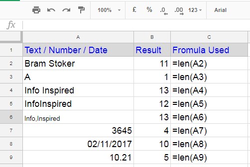
Note: The LEN function will return the count of all characters in the text, even spaces and non-printing characters.
LEN Function in Google Sheets + IF Combination
Assume you have the following formula in cell B1:
=A1*100It returns 0 when A1 is blank. In that case, you want to return blank instead of 0. You can do it mainly in two ways:
=IF(A1<>"", A1*100,)
=IF(LEN(A1), A1*100,)
In these formulas, A1<>"" and LEN(A1) are the logical expressions in the IF function.
Syntax: IF(logical_expression, value_if_true, value_if_false)
The combination of LEN and IF is widely used by Google Sheets users. So, if you see =IF(LEN(reference), read it as =IF(reference<>""
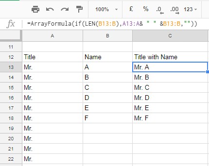
In the following example, I’ve used this combination in an array formula to return the concatenation of titles in cells A13:A and names in B13:B, returning blank if the name is blank.
=ArrayFormula(IF(LEN(B13:B), A13:A& " " &B13:B, ""))The result will be as follows:
Here is an alternative formula:
=ArrayFormula(IF(B13:B<>"", A13:A& " " &B13:B, ""))LEN Function in Data Validation in Google Sheets
You can understand the importance of the LEN function in data validation from the example below.
I want to ensure that all the values in the range C1:C10 are text and 10 characters in length, as those are product IDs and we use 10-character length product IDs.
We can use the following combination of AND, LEN, and ISTEXT functions as a custom formula within data validation as follows:
- Select cells C1:C10.
- Click on Data > Data validation > Add Rule.
- Select “Custom formula is” under Criteria.
- Enter the following formula:
=AND(LEN(C1)=10, ISTEXT(C1)). - Click Done.
Resources
You can find several formulas in this blog that utilize the LEN function. Here are a few tutorials:


=ArrayFormula(if(LEN(B13:B),A13:A& " " &B13:B,""))Why the
len(B13:B)has no condition? I keep trying like yours, but it doesn’t work.Hi, An Dang,
I have updated the post and included “Additional Tips” to answer your question. Please try again.
I have three columns. A = Names, B = Date, C = Answer(Yes/No).
Users can submit the Form each day. But can choose the Answer “Yes” only once a week.
If by mistake, an individual has input “Yes” multiple times within a week, it should be counted just 1 (as a rule, once a week)
I tried your various examples on this site but could not find the solution.
Can you please help me with this problem?
Hi, David,
Make column D empty. Then in cell D1, insert the below formula to return a column with week numbers.
=ArrayFormula({"Week #";if(A2:A="",,weeknum(B2:B22,2))})Now empty the columns E and F. Then in E1, the Query will return the required count.
=query(query(A1:D,"Select A,count(C) where C='Yes' group by A,D"),"Select Col1,count(Col2) group by Col1 label Count(Col2)'Count of Yes'")Does this solve the problem?
For any further assistance on this matter, please share a sample sheet URL below.
I want to find the number of occurrences of, say, “X” within a range of cells, where “X” may occur multiple times within any cell.
Hi, Richard,
Here are two formulas that you can try.
Range: A2:D4
Case-sensitive:
=LEN(regexreplace(textjoin("",true,A2:D4),"[^x]",""))Case-insensitive:
=ArrayFormula(LEN(regexreplace(textjoin("",true,lower(A2:D4)),"[^x]","")))In the expanding count formula, in cells Values, P for present and A for absent values are there. How can I count P or A for each row?
Hi, Suresh Patel,
I think the below MMULT based tutorial fits your requirement.
How to Expand Count Results in Google Sheets Like Array Formula Does.
If not, please share a mockup sheet.