The role of data validation, or you can say data constraints, is to ensure data quality by applying validation logic into spreadsheet cells. I am sharing some of the best data validation examples in Google Sheets.
Have you tried data validation in Google Sheets before? It’s one of the musts to learn features in Google Sheets.
It enables Google Sheets users to create drop-down lists in cells and is also an effective way to validate manual entries.
With data validation, you can control the types of values entered in a cell or cell range.
As I have said above, I am sharing some of the best data validation examples in detail in Google Sheets.
It includes in-cell drop-down lists, validation checkboxes (tick boxes), custom (data validation formula) rules, conditional data validation, etc.
I wish to make this tutorial, i.e., the best Data Validation examples in Google Sheets, one of the best available resources related to it.
The data validation command is available under the Data menu in Google Sheets. Also, you can find part of it (tick box and drop-down) within the Insert menu.
The Best and Must-To-Know Data Validation Examples in Google Sheets
Drop-down is the most commonly used data validation feature in Google Sheets. So let’s begin with it.
How to Create a Drop-Down List in Google Sheets
See some data validation examples in Google Sheets related to the drop-down menu. From that, you can learn how to create a drop-down menu in Google Sheets and its usefulness.
You can create a drop-down list in Google Sheets in two ways. They are;
- Drop-down
- Drop-down (from a range)
How do they differ?
Drop-Down: For Adding Menu Items Manually
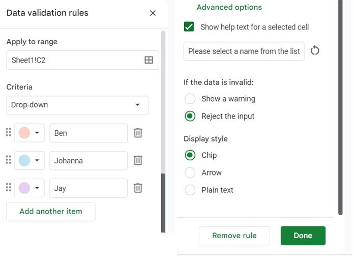
Let’s insert one drop-down menu in cell C1 that contains three names: “Ben,” “Johanna,” and “Jay.”
Here are the step-by-step instructions to insert a simple drop-down menu in Google Sheets.
Steps:
- Go to the cell where you want to create the drop-down menu, e.g., C1.
- Go to the Data menu > Data validation.
- Click the “+Add rule” button.
- Select the “Drop-down” as the Criteria.
- Type the menu items (e.g., “Ben,” “Johanna,” and “Jay”) that you want to appear in the drop-down.
- If you want, you can choose individual colors for each item.
- Click “Done.”
You can use the “Add another item” button to add more menu items and the dustbin icon to delete unwanted items.
Advanced Options:
What to do if somebody hand-enters a name that is not on the list in cell C1?
- You can “Show a warning” but allow entry. A red triangle will appear in cell C1.
- Reject the input outright and show a Help text for the selected cell, i.e., C1.
There are three display styles.
- Chip:- Chip display style helps open the menu by clicking an arrow in the cell.
- Arrow:- Open the menu by clicking on it (Arrow).
- Palin Text:- Double-click on the menu to open it.
Drop-Down (from a range): For Adding Menu Items from a Range
It is the most followed method to insert a drop-down menu in Google Sheets.
In this method, you must enter the menu items in a column, row, or cell range and point data validation to add those items to the drop-down. Here is how.
For example, enter the names “Ben,” “Johanna,” and “Jay” in cells F1, F2, and F3, respectively.
Then follow the above steps (please scroll up to see) 1 to 3. In the fourth step, select Drop-down (from a range).
Enter the range F1:F3 in the given field and click “Done.”
If you want to include more names in the future, you may enter F1:F10 instead of F1:F3. All other settings are the same.
You May Like: Create a Drop-Down Menu From Multiple Ranges in Google Sheets.
Time to go to some best data validation examples in Google Sheets. Let’s start with a chart.
Real-life Practical Use of Drop-Down Menu in Google Sheets
I am using Google Sheets in-cell drop-down menu in the below instances.
Data Validation Drop-Down to Control Charts in Google Sheets
Here is one of the best data validation examples in Google Sheets. See how to control the source data of a chart dynamically.
You can see the drop-down list in cell N1 which controls the Column chart data.
If you want to control your charts (source data) in Google Sheets as above, you can follow this guide – How to Get Dynamic Range in Charts in Google Sheets.
How to Create a Drop-down List Across Sheets in Google Sheets
Can I copy the drop-down list across sheet tabs in Google Sheets?
If you want the same drop-down list in multiple sheets, copy and paste it.
No need to create the same drop-down menu when you want it in multiple cells whether within the Sheet or another Sheet in the same file.
It applies to both Drop-down and Drop-down (from a range).
How to Create a Conditional Drop-down List in Google Sheets
To create a conditional drop-down list in Google Sheets, you can take the help of the functions Filter or Query.
What is a conditional drop-down menu in Google Sheets?
Sometimes you may want a drop-down list conditionally. Better, I will explain it with an example.
Conditional Drop-down Menu Example:
Assume, for example, you want to create a drop-down menu using the Drop-down (from a range) data validation in Google Sheets.
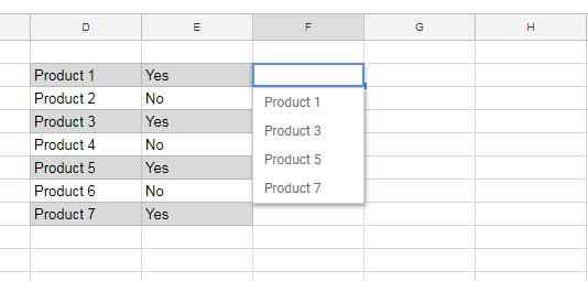
In that, the list is from the range D2:D. You don’t want all the items in this range to appear in the drop-down.
You want only such items in the drop-down if their corresponding values in E2:E is “Yes.”
Here are the steps involved.
Steps to Create a Conditional Drop-down List in Google Sheets:
I am taking the above same sample data for my example.
Apply the below Filter formula in any other blank column. Here I am inserting this formula in cell H2.
=filter(D2:D,E2:E="Yes")Now you can enter H2:H instead of D2:D in the field under the Drop-down (from a range) in data validation in Google Sheets.
Here is another tutorial, in line with the above, as an addition to my best data validation examples in Google Sheets – Distinct Values in Drop Down List in Google Sheets.
It also explains conditional Data Validation in Google Sheets but from a different angle.
Drop-Down List That Is Dependent on Another Drop-Down List
First, I thought I shouldn’t include this tip in this tutorial which features the best data validation examples in Google Sheets.
There is no built-in flexible solution to create a dependent data validation drop-down in Google Sheets other than using an Apps Script.
But, in a limited way, you can create a dependent data validation drop-down menu in Google Sheets.
Example to Data Validation Dependent Drop-down List:
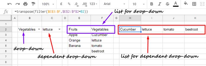
In cell B2, you can see a drop-down menu. In cell C2 there is another drop-down menu dependent on the first one.
That means when you select “Fruits” in the first drop-down, the second drop-down will only list fruit items.
If the selection in the first drop-down is “Vegetables,” the second one will list vegetables only.
That means the first drop-down list contains categories, and the second one, the items coming under each category.
Steps to Create a Data Validation Dependent Drop-down Menu in Google Sheets:
I think here I must illustrate the procedure first.
Steps:
- Enter a few fruit names in the range E2:E. The title in E2 should be “Fruits.”
- Similarly, enter a few vegetable names in the range F2:F. Cell F2 should contain the title “Vegetables.”
- You should enter E2:F2 in the field under the Drop-down (from a range). I’ve already explained the steps to create a drop-down menu in Google Sheets. Please scroll up and see.
- Insert the below formula in cell H2 and use its output in the range H2:2 as the second drop-down’s (drop-down in cell C2) range.
=transpose(filter($E$3:$F,$E$2:$F$2=B2))That’s all you want to do to create a data validation dependent drop-down list in Google Sheets.
Here find a more detailed tutorial on this topic – Multi-Row Dynamic Dependent Drop-Down List in Google Sheets.
In addition, to know the functions I have used, please check this guide – Google Sheets Functions Guide.
Data Validation Examples in Google Sheets Using Checkboxes (Tick Boxes)
How to Insert Data Validation Checkboxes in Google Sheets?
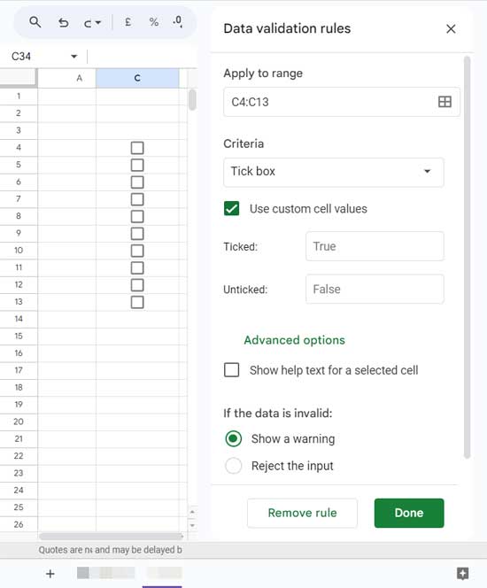
Data Validation supports Checkboxes. You can insert tick boxes in two ways.
Go to the Insert menu and click on the Tick box or go to Data > Data validation > Add rule > Criteria > Tick box.
I prefer the former method even though the latter offers a few advanced tick box options.
What are they?
Show a warning or reject input with help text similar to the drop-down.
Also, you can replace the underlying Boolean TRUE (ticked) or FALSE (unticked) values with custom cell values. Didn’t get it?
Checkboxes are interactive, which means they are clickable. You can click and unclick a checkbox.
When clicked a tick box, the value in that cell will be TRUE, or else FALSE. Instead of TRUE or FALSE, you can set any custom value.
Additional Resources Related to Tick Boxes in Google Sheets:
- Check-Uncheck a Tick Box based on the Value of Another Cell in Google Sheets.
- 10 Best Tick Box Tips and Tricks in Google Sheets.
- Change the Tick Box Color While Toggling in Google Sheets.
- Tick Mark: Lock and Unlock Cells Using Checkboxes in Google Sheets.
- Assign Values to Tick Box and Total It in Google Sheets.
Restrict or Constrain Cell Value to Number, Date, or Text Using Data Validation
At the beginning of this tutorial, I mentioned the purpose of data validation in spreadsheet applications. It’s to ensure the data quality by applying validation logic to cells.
I have already provided you with a few possibly best data validation examples in Google Sheets.
No doubt, all are related to drop-downs and checkboxes.
Some simple data validation settings can ensure maximum data quality with minimum effort in Google Sheets. Here are a few of them.
Data Validation in Google Sheets to Limit or Apply Constraints to Entry of Numbers
You can easily set certain constraints to entering numbers in a cell or range of cells.
Let’s see how to limit or apply some constraints to entering numbers in a selected cell or cell range.
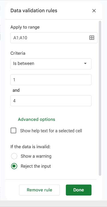
Assume, for example, your company has certain restrictions set for sanctioning overtime (OT) hours. The minimum is 1 hour, and the Maximum is 4 hours a day.
So, while entering daily overtime data in Google Sheets, you want to ensure that Sheets permits only entering numbers >=1 and <=4 in the set range.
Here is how to do that.
Select the cell or cell range, e.g., A1:A10, where you want to enforce or assign some data entry constraints related to numbers.
Then go to the menu Data > Data Validation > Add rule.
Under Criteria, select “Is between” and enter the numbers 1 and 4 as shown below.
Here are all the number-related criteria in data validation in Google Sheets.
- Greater than.
- Greater than or equal to.
- Less than.
- Less than or equal to.
- Is equal to.
- Is not equal to.
- Is between.
- Is not between.
Data Validation in Google Sheets to Limit Date Entry
Set some constraints in a cell or range of cells about Date entry. It ensures that we enter or pick correctly formatted dates or enter dates that fall within a given range.
To set, choose the Data Validation “Criteria” as one of the following.
Available Criteria:
Is a valid date: It ensures you enter or pick a valid date, not a text or number.
Related: How to Get Date Picker in Blank Cell in Google Sheets.
Other Date Criteria: Date is, Date is before, Date is on or before, Date is after, Data is on or after, Data is between, and Date is not between are the other criteria.
Limit Text Entry in Google Sheets Using Data Validation
You may want only valid email IDs under the title “Email” in an employee database. Then apply the “Text is valid email” criteria as shown below.
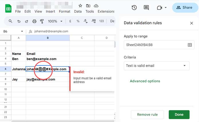
It’s another way to ensure the quality of data in Spreadsheets.
Other Text Criteria: Text contains, Text does not contain, Text is exactly, and Text is valid URL are the other available text criteria options.
Use them as per your requirement.
Custom Formula-Based Data Validation Examples in Google Sheets
With the “Custom formula is” criterion in data validation, we can improve the data cleansing capability of Google Sheets.
In Google Sheets, just like the custom formulas in conditional formatting, the absolute and relative cell references play a vital role when using a custom formula in data validation.
The Role of Relative and Absolute Cell References in Data Validation
Relative and Absolute are the two types of cell references in Google Sheets. How do they differ? I’ll explain it in a nutshell.
Definitely, I am going to give more priority to how to use the data validation custom formula in Google Sheets. But for that, you must understand the said two types of cell references.
Relative Cell References:
When you copy a formula to another cell, the cell references in the formula also move if they are relative.
Example: =C1
Absolute Cell References:
We can control the behavior of cell references using Dollar signs.
Dollar signs play a vital role in absolute cell references.
If you use Dollar signs with a cell reference, when you copy, its cell reference remains constant in a particular way. See the examples.
Example:
=$C$1: Row and column remain constant.
=$C1: Row changes.
=C$1: Column changes.
My ultimate goal with this Google Sheets tutorial is to provide you with some of the best available data validation examples in Google Sheets. So here we go.
I will use relative and absolute cell references in the below custom formula-based data validation examples.
Conditional Data Validation in Google Sheets Using Custom Formulas
Let me start with a basic example. Let’s see how to use custom formulas in data validation in Google Sheets.
Allow Data Entry in a Range (A1:A5) if Adjoining Column (B1:B5) Contains “Yes”:
Here I am applying a custom formula to the range A1:A5.
A1 will be validated if B1 is “Yes,” A2 will be validated if B2 is “Yes,” and so on.
Steps:
- Select the range A1:A5.
- Go to the Data menu Data Validation > Add rule.
- Select “Custom formula is” under Criteria.
- Enter the below formula.
=B1="Yes"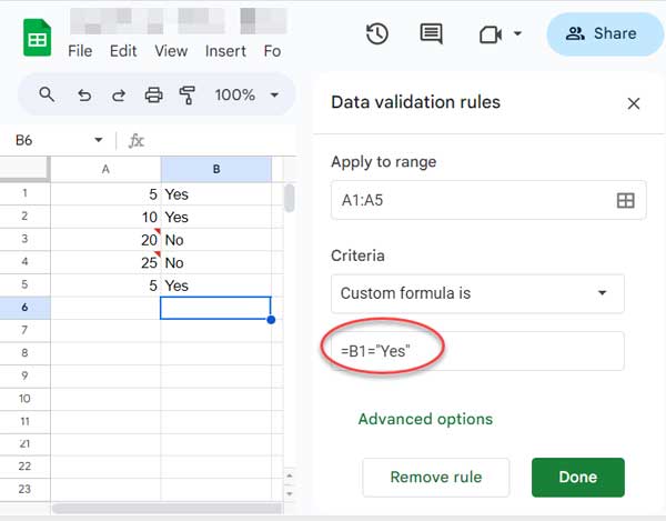
The above formula is an example of relative cell reference in data validation in Google Sheets.
Just test it on your Sheet to understand the behavior.
Here are a few more custom-formula-based best data validation examples in Google Sheets.
Restrict or Allow Odd or Even Numbers in a Range:
How to allow only odd numbers in a range?
I am applying this rule to the range A1:B10. So enter A1:B10 in the “Apply to range” field in the “Data validation rules” panel.
=isodd(A1)How to allow only even numbers in a range?
=iseven(A1)Conditionally Allow ODD or EVEN Numbers in a Range:
I want to allow only even numbers in the range A1:A5 if the range B1 contains TRUE.
To set the rule, select the range A1:A5 and use the below customer formula in data validation.
=and(iseven(A1),$B$1=TRUE)Replace ISEVEN with ISODD to allow only odd numbers when B1=TRUE.
I’ve used both relative and absolute cell references in the above conditional data validation example in Google Sheets.
Data Validation to Restrict Duplicates in Google Sheets:
You can restrict the entry of duplicates in Google Sheets using the data validation custom formula feature. Read that here – How Not to Allow Duplicates in Google Sheets.
Further, I have a tutorial that details how to use Regex in data validation in Google Sheets – Restrict Entering Special Characters in Google Sheets Using Regex.
Time to wind up this tutorial on best data validation examples in Google Sheets. Please post your views in the comment. Enjoy!


Hi and thanks!
Is it possible, like in Access, that the combo box (validation dropdown) shows a text and stores a number?
Data Validation Shows and select: Oranges, but store no 2 in the cell?
Fruits | Fruit Id
Apples | 1
Oranges | 2
Bananas | 3
Hi, Andrés,
That is not possible. But in the next cell, we can use a formula for that.
=vlookup(A1,{"Apples",1;"Oranges",2;"Bananas",3},2,0)A1 refers to the drop-down box.
Hi Prashanth,
Thanks in advance for your help.
Is it possible to have a drop-down list only if another cell has a specific value, otherwise it will be free from the text?
Hi, jay c areh,
As far as I know, that is not possible right now using a formula (logical test). Maybe possible to use Apps Script. But I am not familiar with it.
Hi Prashanth,
Very nice explanation.
I am curious as to, is there a method of obtaining the nth value in the drop-down list without using lookup, etc.
Hi, Manoj Gupta,
It may be possible if you use “list from a range” in data validation.
Eg.:
List from a range:
=$G$3:$G$13Formula:
=filter(G3:G13,row(G3:G13)=9+2)Thank you for these wonderful tips!
I want to use data validation. Any idea, how one could enforce a user to enter data from a list in the order of that list?
It is allowed to enter an item multiple times. For example:
chapter1
chapter2
chapter2
chapter3
…
It should not be allowed to enter chapter3 after chapter1:
chapter1
chapter3 –> not allowed
They must first enter chapter2…
Thank you in advance!
Best regards,
Jurgen L.
Hi, Jurgen L.,
It can be possible if you only let the user input the values via a drop-down list.
In my next post, I’ll elaborate on my idea. I’ll get back to you here!
Best,
Hi, Jurgen L.,
Here is my attempt to solve your problem – Data Validation to Enter Values from a List as per the Order in the List in Google Sheets.
I hope that helps?
Hi Prashanth,
Perfect! Exactly what I was looking for. I have 2 comments on this, but I will put those under the specific post.
Thank you!
Jurgen L.
Excellent as always, thank you for your comprehensive work.
Could you offer any tips for a Sheet I’m creating for a budgeting exercise?
-Basically, I want users to check tick boxes to indicate the products they want to buy.
-I want the sheet to subtract the total cost of the checked products from a ‘Budget’
-I want the sheet to prevent users from checking any products that would cause the budget to be negative.
I’ve got the first two parts working, but I can’t figure out the Formula for the Data Validation.
Example below. The goal is if users checkbox Apple, budget changes to $2. Then if they checkbox Orange, budget changes to $0, but if they then try to checkbox Banana as well, they’ll get an error because $3>$0.
Budget $3
FALSE Apple $1
FALSE Orange $2
FALSE Banana $3
FALSE Carrot $4
Hi, David Markey,
As far as I know, you can’t control a tick box with another data validation in Google Sheets. Because the cell containing the tick box will overwrite any other data validation rule. The tick box itself is a data validation item.
I suggest you a workaround with conditional formatting.
Example:
The cell range C2:C5 contains the fruit names and the adjoining cells to the right, i.e. D2:D5 contains the checkboxes (tick boxes). The dollar amount 1 to 4 is in the range E2:E5.
Now enter the budget amount $3 in cell E8.
Select D2:D5 and go to Format > Conditional format. Then select “Custom formula is” below the “Formula rules”.
In the provided field (blank by default), insert the below formula.
=and(D2=TRUE,$E$8-sumif($D$2:$D$5,TRUE,$E$2:$E$5)<0)It will highlight all the ticked boxes once the budget goes less than 0. It will alert the user.
Hi Prasanth
I have a challenge with doing data validation with 2 dates.
Date 1 is the start date and that is selected from a drop-down list (result in B2).
In B3 I want the user to put end date where the end date can be >= start date but not before. How can I ensure this?
Hi, Jonathan.
Please follow this screenshot for the correct validation settings.
So I am trying the technique given above for using a filtered range to add a dropdown contingent on another dropdown. I am trying to get it to work on multiple rows, however, when the rows get sorted, the data validation doesn’t follow suit and adjust the range that it is looking at, even though the formulas (and everything else) does. I’ve tried it multiple different ways, and it seems that data validation by range never seems to follow the same sorting logic as formulas and conditional formating.
I am trying to restrict data from being entered into a range of cells based on two different rules.
My range is E3:P3 and my checkbox is in D3. Currently if D3=False, then you can not enter data, which is perfect.
However, I have a feature in column T that has a running clock essentially counting down from 24 hours. When it hits 0:00:00, it changes to “Auction Ended”.
I would like to be able to restrict entry into the range E3:P3 when “Auction Ended” is reached in T3 as well.
Is there a way to add an “or” option in the custom formula data validation field, or can I make the checkbox = “False” upon T3 equalling “Auction Ended”.
Hi, Joseph Melanson,
The formula that lets you only enter values in the range E3:P3 if the checkbox is unchecked and the value in T3 is equal to “Auction Ended”.
=and($D$3=false,$T$3="Auction Ended")=falseYou can make it a more strict rule by changing AND logical operator with OR as below.
=or($D$3=false,$T$3="Auction Ended")=falseI Think this second rule is what you are looking for?
Thanks for the info!
My issue is that the data validation seems to always use the absolute reference even without including the $. I just want to copy my data validation down a column and have the custom range come from other columns in the same row the same way a formula copies relative cell references.
Same issue. If I use “List of range” in Data validation then it always uses the absolute reference regardless of the
$. Relative reference works when I use “Custom formula” in Data Validation. Maybe this is a bug?Hi, Soo Gee,
It’s doesn’t seem like a bug. Google Sheets development team has to work on it. In my personal opinion, the data validation (especially the drop-down) is not as flexible as in Excel.
Hi Prasanth.
Great article 🙂
I have two questions.
1. I have a sheet (Sheet1) showing dropdowns based on a column from another sheet (Sheet2). So I use data validation to show the dropdown based on a list from a range fx. “Sheet2!A2:A50”.
In Sheet2 column B, I indicate if the data is active or not using “Yes” or “No”. The dropdowns in Sheet1 should only show data from Sheet2 column A if the data in column B is set to “Yes”.
I have to use the option “Custom formula is” but what should the formula be?
I tried combining your examples and used:
Sheet2!A2:A50=$B="Yes". But it doesn’t work and no dropdown is shown.2. Can I keep the formatting from the cells I use for the dropdown data? So if I in Sheet1 choose a value in the dropdown the font, font color and cell background color from the cell in Sheet2 is shown in Sheet1?
Hope you are able to help.
Best
Casper
In Sheet2 cell D2, insert the following FILTER formula which filters column A if column B=”Yes”.
=filter(A2:A,B2:B="Yes")In Sheet1 Data validation you must use “List from range” instead of ‘Custom formula is” as ‘Custom formula is’ not for drop-down list.
Select the range ‘Sheet2!D2:D’ in the provided validation field.
At present, cell formatting won’t be retained in data validation.
I hope this helps?
It helped a lot and works now.
Thanks for the help Prasanth 🙂
I am trying to find a way to check if the data entered by users in the date column is in the following format
mm/dd/yyyy hh:mm:ss.I used the custom formula in data validation
=IF(NOT(ISERROR(TEXT(D22,"mm/dd/yyyy")&TEXT(D22,"hh:mm:ss")))),"valid date","invalid date"), but it doesn’t work.Thanks in advance.
Hi, Kareem,
I have two solutions.
=AND(ISDATE(D22),D22-INT(D22)>0)The above formula in Datavlidation requires a time component (date-time) to validate the cell.
For example, the date entered as 11/04/19 00:00:00 will be rejected but 11/04/19 00:00:01 will be accepted.
The second option just allows date entry using the Data validation criteria set to Date > Is a valid date.
Then format the entered date to Timestamp from the Format menu Number > Date Time.
Best,
Thank you! the article was really helpful.
But is there a way that allows me to execute formulas for some cells only while the formulas in other cells do not execute dynamically on changing the source file?
Like if I write all the formulas that I want to apply only in the column with values of October only while keeping all the values for past and future months undisturbed.
I hope I have made my issue clear and in case there is something not clear please revert back.
Thanking you in Anticipation.
Regards.
Hi, Nur Ali,
Nope! I didn’t understand your question. Will you be able to share a copy/example sheet?
Best,
Hi,
Thanks for the tutorial, it’s been a great help!
I need to replicate your “drop-down menu dependent on a drop-down menu”, however, I need to to this not once but like 150 times. (I want to create a table for invoices, where every line has a drop-down menu for “department” and one for “position” dependent on “department”).
So I initially thought I could just paste down what you have in H2:2 and paste down the data validation fields as well. However, as you said earlier, if you paste down the data validation, the references do not change.
As a result, my second drop-down menu always shows the same available positions in every line rather than changing dynamically based on what department I chose in that line.
Any idea how to fix this?
Hi, Andy,
I have provided a link to another detailed tutorial, the title starting with “Multi-Row Dynamic D…”, under the sub-title which you have mentioned. Please check that for more details on the multi-row depended drop-down list with the said limitations.
Best,
Wonderful material. Thanks for the teachings .. migrating from Excel to Google Sheets.
Hi, your posts are brilliant thank you. I am looking for some help.
I want the drop-down list to pick up different ranges based on the information displayed in another cell.
For example if cell A1 displays the information ‘rural’ I want it to pick up the range for Rural. If it displays ‘suburban’ I want it to pick up the range for Suburban. Is this possible?
Thanks,
Simon
Hi, Simon,
That’s possible with a helper column.
Name different ranges using the menu Data > Named ranges
For example, I am naming the range H3:H13 as ‘rural’ and I3:I13 as ‘urban’
In J3 enter this formula.
=indirect(A1)This will populate data based on the value in cell A1. This is my helper column to create the drop-down.
I mean in Data > Data validation > List from range > select J3:J13.
See if that works for you?
Best,
I am trying to find a way to create a list of data validation and once an item is selected in a column it cannot be selected again. Using it for booking available horses for our riding lesson program. So I select the horse from a drop-down list and he is not available in the next cell down. but can be selected in the next column.
Hi, Rebecca Rainey,
You can find something similar here – Distinct Values in Drop Down List in Google Sheets
If you want any further clarification, feel free to ask in the comment section below in that tutorial along with a link to your demo Sheet.
Best,
Thank you, Prashanth for your help.
The issue is, when I use this Indirect formula in a cell, it displays the ítems below that cells. But I want the ítems to appear in a drop list.
Something like in MS Excel, where I can fill on the data validation list with the formula (indirect (A2)) and it is allowed.
Best regards,
Hi, JM,
Google Sheets doesn’t support this.
I have detailed that under the sub-title “Indirect in Drop-down List in Excel and Sheets” in my Indirect Excel-Sheets comparison.
Comparison: Indirect in Excel vs Indirect in Google Sheets
Oh, Thank you for you support.
Best,
Excuse me, can I use function INDIRECT into an option “list of ítems” from a data validation?
I would like, depending on the value that I choose from a list in Column A, that in column B display a drop-down list with some values that I has been loaded with the option “Name Ranges”.
Thanks for the help that you can give me.
Hi, JM,
Assume, you have a drop-down list in cell A2 in “Sheet1” with the items “Books” and “Sports”.
In “Sheet2” in column A enter the book names. In column B in that sheet enter the sports items. Name (DATA > NAMED RANGES) these lists as “Books” and “Sports” respectively.
In cell B2 in Sheet1 you can use the below Indirect formula.
=indirect(A2)Best,
I have a sheet with a data validation column where the end user selects a numeric value from the drop-down. The criteria in data validation are the “list of items”.
I have a separate cell that collects the sum of all cells in that column.
Problem is that the sum remains at 0. It’s not working.
Any thoughts of how to collect the sum of the selected values used in the data validation column?
Hi, Jim,
If you want me to help you to identify the problem, please replicate it in a sample Sheet and share.
Best,
I want to restrict a value in a cell based on another cell in the same row.
A B
4 9 – allowed
5 0 – allowed
6 5 – the value in A should not be allowed
The value in A must not exceed what is in B. If the value in B is zero, any figure is allowed in A
How to set up data validation for this in column A
Hi, Arul Selvan,
I assume you have the above values in A1:B. Select the range A1:B and use the following custom data validation formula.
=or(LT(A1,B1),B1=0)Best,
Very useful article and example,
I tried and thought about your data validation custom formula example, but I am not able to figure out how to set up a drop down in column B that adapts to the selection in column A. And then have this replicated till row # 500 or so.
Can you help me out on this?
Hi, Shyam,
I have detailed at the beginning of this tutorial how to create a drop-down menu using the methods ‘List from Range’ and as well as the ‘List of Items’ methods.
Create a drop-down menu using the ‘List from Range’ method in cell B1. You can then copy this drop-down and paste to the range B2:B500.
Please do note that the cell reference (criteria reference) in the data validation won’t change. It’ll be the same for all the data validation drop-downs.
Best,
Prashanth KV
I had the same issue. Not sure if yours is solved but for others here is a link to the script!
https://support.google.com/docs/thread/22008388?hl=en&authuser=2&msgid=22017112
Hi – great article, thanks. Unfortunately, whatever I do I can’t get a dropdown to recognize a blank cell as an option – it just misses it out. Any ideas on how to include this?
Thanks
Ash
Hi, Ash,
When you first create a drop-down menu, you may have noticed that by default the cell contains the drop-down menu is set to blank. But once you select an item you won’t get an option to select blank again. I mean set the cell that contains the drop-down menu to blank.
To make it blank again, just hit the delete button on the cell contains the menu.
Best,
If in a sheet I have one tab that is my ‘data sheet’ eg columns named Product, Colour, Year, Price and have these all completed. In another tab I want to do a product list when I visit a client – so I have data validation dropdowns for completing Product, Colour and Year. Am I then able to have the Price auto-filled from the ‘data sheet tab’? Thank you for any suggestions.
Hi, Tiffany,
I think, Yes!. You can use Vlookup to lookup the product.
Assume the above data in the “data sheet” is in A1:D and row # 1 is the header row.
In another tab, you have the following values (via drop-down).
A1 – product
B1 – color
C1 – Year
In D1 you can use the Vlookup as below.
=ArrayFormula(vlookup(A1&B1&C1,{'data sheet'!A2:A&'data sheet'!B2:B&'data sheet'!C2:C,'data sheet'!D2:D},2,0))Want to know more about this Vlookup combined criteria use?
How to Use VLOOKUP with Multiple Criteria in Google Sheets
Best,