How to Use the FILTER Function in Google Sheets

The FILTER function in Google Sheets filters rows or columns based on conditions. It provides several benefits, and here are a few advantages of this function:

Troubleshooting Formula Errors: The FILTER function helps troubleshoot formula errors. For instance, if a SUMIFS formula does not return the correct result, you can filter the range based on the same criteria or part of the criteria and examine rows to identify the issue.
Selective Data Attention: Filtering enables you to concentrate on or highlight the essential data by isolating it based on specific criteria.
Improved Formula Performance: When utilizing open ranges in formulas, employing FILTER to eliminate blank rows and columns can enhance the performance of the formulas.
Creating Category-wise Tables: We can create multiple tables based on specific criteria by filtering categories.
As a Custom Function in Lambda: FILTER plays a significant role in the REDUCE function when joining tables in Google Sheets (Master Joins in Google Sheets (Left, Right, Inner, & Full) – Duplicate IDs Solved)

Syntax and Arguments

Syntax of the FILTER Function in Google Sheets:

FILTER(range, condition1, [condition2, ...])

Arguments:

range: The data range to be filtered vertically or horizontally.
condition1: A row or column that evaluates to TRUE or FALSE values using a criterion.
condition2: Additional rows or columns that evaluate to TRUE or FALSE values using criteria.

An example of condition1 is A3:A="Apple", which will return TRUE for matching rows, otherwise FALSE.

In formulas, you may encounter instances where only a range, such as A3:A, is used as condition1, condition2, etc. This typically relates to filtering a numeric or date-type column. In such cases, it interprets numbers/dates as TRUE and treats blank/zero cells as FALSE.

Basic FILTER Function Examples in Google Sheets

For testing the FILTER function, we will use sample data that contains the World Cup Football title winners since 1930.

The data is arranged in columns A, B, and C, where A1, B1, and C1 contain the field labels “Year,” “Hosts,” and “Winners,” respectively.

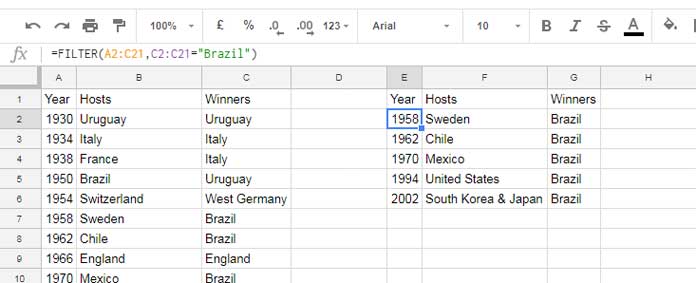
Basic Example: Filter Function in Google Sheets

To filter the range for matching “Brazil” in the Winners column, you can use the following formula:

=FILTER(A2:C, C2:C="Brazil")

How does the FILTER function work in Google Sheets?

In this formula, A2:C represents the range. The condition1 is C2:C="Brazil", which would return TRUE wherever the condition matches.

Additional Notes

If you enter the above condition1 as a separate formula in a cell, it won’t return TRUE/FALSE. In standalone use, you must enter the formula as an ArrayFormula like:

=ArrayFormula(C2:C="Brazil")

Inside the FILTER function, there is no need to use the ArrayFormula function.

In the FILTER function in Google Sheets, the column that contains the condition can also be outside the filter range.

For example, see the below formula where the condition is in the range C2:C, which is outside of the filter range of A2:B:

=FILTER(A2:B, C2:C="Brazil")

Mastering Multiple Criteria Usage in the FILTER Function Google Sheets

If you intend to employ multiple criteria in the FILTER function, it’s crucial to understand a key calculation, as the FILTER function requires a row or column with TRUE or FALSE values as conditions. The value of TRUE is equal to 1, and FALSE is equal to 0.

So, when using multiple criteria, consider the following calculations:

condition1 + condition2: This will return >=1 if either or both of the conditions are TRUE.
- TRUE + TRUE = 2.
- TRUE + FALSE = 1.
- FALSE + TRUE = 1.
- FALSE + FALSE = 0.
condition1 * condition2: This will return 1 only if both conditions are TRUE.
- TRUE * TRUE = 1.
- TRUE * FALSE = 0.
- FALSE * TRUE = 0.
- FALSE * FALSE = 0.

Now, you know when to use the + operator and when to use the * operator with conditions. If not, refer to the following examples.

Example #1: All Conditions are TRUE

How do we extract the records corresponding to the title winner Brazil after 1990?

We can use the formula in two ways:

=FILTER(A2:C, A2:A>1990, C2:C="Brazil")
=FILTER(A2:C, (A2:A>1990) * (C2:C="Brazil"))

This is because we want to filter the range based on conditions from two different columns, and both of them evaluate to TRUE.

The following formulas filter the range A2:C if the year in column A (A2:A) is greater than or equal to 1950 and less than 2000.

=FILTER(A2:C, A2:A>=1950, A2:A<2000)
=FILTER(A2:C, (A2:A>=1950) * (A2:A<2000))

Example #2: Any of the Conditions is TRUE

Filter the range for the World Cup title winners Brazil and Spain.

=FILTER(A2:C, (C2:C="Brazil") + (C2:C="Spain"))

Since both conditions are from the same column, we want to evaluate either of the conditions to TRUE in a row.

To extract the range if either the host or winner is Brazil, you may use this formula:

=FILTER(A2:C, (B2:B="Brazil") + (C2:C="Brazil"))

Hardcoded Conditions vs Cell References

In all the above examples, we hardcoded the conditions within the FILTER function. Alternatively, you can enter the criteria within cells and refer to those cells in the formula.

In the following sample data in the range A1:E, the data types in each column are text, date, number, TRUE/FALSE, and date. They are Name, Date of Birth, Age, Tick Box (Membership Status), and Valid Until.

The cells H1, H7, and H13 contain a date, a number, and the Boolean value FALSE as the criteria. You can directly use the cell references inside the formula. Please refer to the screenshot below.

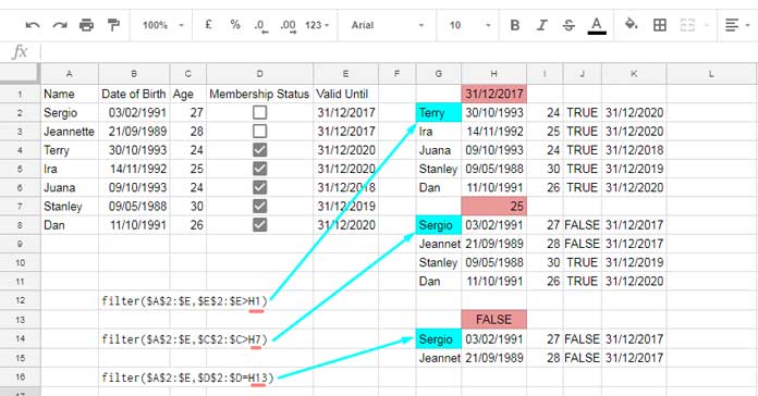
Using Cell References in FILTER Function: Example

Note:

When hardcoding the date criterion within the formula, please use the DATE function in the syntax DATE(year, month, day).

For example, if you want to match 31/12/2017 in column E, the condition will be E2:E=DATE(2017, 12, 31)

Advanced FILTER Function Examples in Google Sheets

If you have completed the above examples, let’s spend some time on the advanced use of the FILTER function in Google Sheets.

Regular Expressions

The easiest way to apply multiple text conditions in a single column is by using REGEXMATCH in the FILTER function in Google Sheets.

The following formula will filter the range A2:E if A2:A contains either of the names Sergio or Terry:

=FILTER(A2:E, REGEXMATCH(A2:A, "Sergio|Terry"))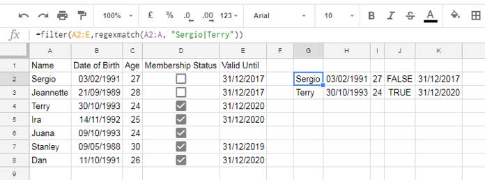

Regular Expressions and FILTER Function: Example

The above formula will partially match the names. To ensure an exact match, you may use this one:

=FILTER(A2:E, REGEXMATCH(A2:A, "^Sergio$|^Terry$"))

Both formulas are case-sensitive. To make them case-insensitive:

=FILTER(A2:E, REGEXMATCH(A2:A, "(?i)^Sergio$|^Terry$"))

You can add more conditions to this by separating each condition with a pipe.

SEARCH and FIND Functions

If you study the above FILTER function examples that use REGEXMATCH, you can easily filter based on partial matches (case-sensitive or insensitive) in a column.

But if you are not yet ready to use regular expressions, you can then use SEARCH (case-insensitive) or FIND (case-sensitive) within the FILTER function.

=FILTER(A2:E, SEARCH("Sergio", A2:A)) // case-insensitive
=FILTER(A2:E, FIND("Sergio", A2:A)) // case-sensitive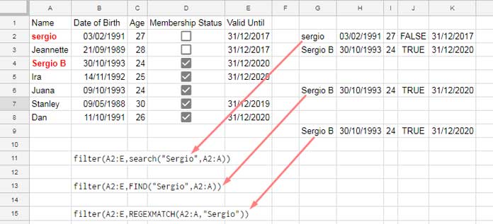

Partial and Case-Sensitive Filtering in FILTER Function: Example

FILTER Function to Filter Columns in Google Sheets

In all the above examples, we have used the FILTER function to filter rows. Similarly, we can filter columns too.

For example, you can use the following formula to filter columns that have the field labels Jan, Feb, and Mar. The table range is A2:G.

=FILTER(A2:G, (A2:G2="Jan") + (A2:G2="Feb") + (A2:G2="Mar"))
=FILTER(A2:G, REGEXMATCH(A2:G2, "Jan|Feb|Mar"))

These formulas will filter the columns in the range A2:G based on whether the field labels in A2:G2 match Jan, Feb, or Mar.

Resources

This tutorial covers everything you need to master the FILTER function in Google Sheets. Below, you can find the usage of this function in conjunction with other functions and also some advanced tips.

40 COMMENTS

Charlotte Gillingham July 29, 2022 At 6:44 pm

Hi, I have the formula

=iferror(filter(Sheet2!$B$1:$N$1,Sheet2!$B$13:$N$13= large(Sheet2!$B$13:$N$13,1)),"")

which finds the largest value in row 13 and returns the corresponding text in row 1.

Is there a way to get it to look at a row based on the contents of another cell (i.e., I don’t know which row the desired data is in, it won’t always be in row 13)?

So if cell A4 in my current sheet contains the word ‘Glasgow,’ find it in column A of sheet2, find the largest value in that row, then return the text in row 1.

I know I need to replace the Sheet2!$B$13:$N$13 element but not sure what to change it to.

- Prashanth July 31, 2022 At 9:44 am
  
  Hi, Charlotte Gillingham,
  
  Thanks for your clear-cut explanation of the problem.
  
  From my test, you require to replace that element with the following one.
  
  filter(Sheet2!B2:N,Sheet2!A2:A=A4)
  
  So the formula would become;
  
  =filter(Sheet2!$B$1:$N$1,filter(Sheet2!B2:N,Sheet2!A2:A=A4)= large(filter(Sheet2!B2:N,Sheet2!A2:A=A4),1))
  
KC April 23, 2022 At 1:51 pm

Hi Prashanth,

Sorry if you already went over this in the article or other comments, and I missed it.

I need to filter using multiple conditions. However, not all of them are always used.

My table might look like this (Sheet1):

Date | Location | Price
1/1 | CA | $25
1/1 | NY | $10
3/4 | CA | $10

Entering the filter information like this (Sheet2):

Date | Location | Price
3/4 | CA | $10

Formula:

=FILTER(A2:C4,A2:A4=Sheet2!A2,A2:C4, B2:B4=Sheet2!B2,A2:C4,C2:C4=Sheet2!C2)

But, if I entered my filter information, leaving one or more of the columns blank, the formula would return N/A.

Date | Location | Price
| CA |

How would you change the formula so it only uses the information that isn’t blank?

Thank you!

- Prashanth April 24, 2022 At 10:21 am
  
  Hi, KC,
  
  First of all, your given formula seems incorrect to me. It should be;
  
  =FILTER(A2:C4,A2:A4=Sheet2!A2,B2:B4=Sheet2!B2,C2:C4=Sheet2!C2)
  
  Regarding your requirement, you can try this.
  
  =FILTER(A2:C4,if(len(Sheet2!A2),A2:A4=Sheet2!A2,row(A2:A4)), if(len(Sheet2!B2),B2:B4=Sheet2!B2,row(B2:B4)), if(len(Sheet2!C2),C2:C4=Sheet2!C2,row(C2:C4)))
  
  You can find a similar tutorial here – Select All or a Specific Category in Multiple Columns in Filter in Google Sheets.
  
Jim December 11, 2021 At 10:38 pm

Hi Prashant,

I need to do data validation using a drop-down list in a cell but the items in the list are selected from a range in another worksheet.

That is easy just using the menu system except it selects matches for the drop-down list based on matching the text string entered starting from the beginning of the validation range items rather than according to content anywhere in the string.

Therefore if I enter “abc” in the cell being validated, the drop-down list will contain “abcxyz” but not “xyzabc” which is what I want.

How can I do this?

- Prashanth December 12, 2021 At 9:11 am
  
  Hi, Jim,
  
  If cell F6 contains “xyzabc” or any other string, you can validate it using either of the below formulas.
  
  Case Insensitive:-
  
  =ifna(match("*abc*",F6,0)>=1,FALSE) =IFERROR(search("abc",F6)>=1,FALSE)
  
  Case Sensitive:-
  
  =IFERROR(find("abc",F6)>=1,FALSE) =regexmatch(F6,"abc")
  
mikapi December 22, 2020 At 9:05 pm

Thanks for these explanations.

I think a case is not covered, (and I am stuck on it).

It easy to filter rows with several conditions which applied to the same range, but how is it possible to filter rows from the result of the first conditions.

I have no success to do that with imbricating FILTER functions.

The problem occurs when trying to obtain one row in a google forms response sheet, based on two columns (one criterion and the time stamp), to extract the last row (in time).

By example:

name | order | apple | lemon | pear
jean | 1 | 2 | 3 | 4
alfred | 2 | 8 | 9 | 10
fred | 3 | 26 | 15 | 16
fred | 4 | 20 | 21 | 22
toto | 5 | 4 | 27 | 28

I would like to extract the number of lemons that have bought “Fred” the second time (maximal order).

- Prashanth December 23, 2020 At 8:39 pm
  
  Hi, mikapi,
  
  You can try a SORT and FILTER combination.
  
  As per your example dataset, there are 5 columns. But from your explanation, I could understand that there are 6 columns and the first column is the timestamp column.
  
  Assume the range is A1:F, then try the below formula.
  
  =ARRAY_CONSTRAIN(filter(filter(sort(Sheet1300!A2:F,1,0), Sheet1300!A1:F1="Lemon"),sort(Sheet1300!B2:B,Sheet1300!A2:A,0)="Fred") ,1,1)
  
  Replace Sheet1300 with the sheet name that contain the data.
  
  If not working, try to share a sheet that contains mockup data.
  
Brian September 22, 2020 At 9:00 pm

Hi Prashanth! I love your tutorials!

I’m having an issue I hope you can help with:

I have a spreadsheet that is doing a nice job of filtering a dataset from another tab. To the right of the columns that show the filtered set, I need to manually hard key new data.

However, if the dataset tab is sorted, it resorts my filter columns, but not my hard key columns. Now the data is mismatched.

Is it possible to make all columns in my filtered tab sort together when the filter columns sort?

- Prashanth September 23, 2020 At 10:50 am
  
  Hi, Brian,
  
  It’s hard to explain. you may find something similar here –
  
  Align Imported Data with Manually Entered Data in Google Sheets.
  
  – and also a video tutorial on the video popup window.
  
Daniel Sef February 27, 2020 At 7:50 pm

Hi, I have a formula …

=SUM(FILTER('INCOME REPORT'!$B$2:$B$999,TO_TEXT('INCOME REPORT'!$C$2:$C$999)="Alex Wages",'INCOME REPORT'!$A$2:$A$999>=VALUE("2020-01-01 00:00:00"),'INCOME REPORT'!$A$2:$A$999<=VALUE("2020-01-31 23:59:59")))

… which works great for January but then when I drag it into February it stays the same is there. Any way to make the dates relative so when I drag the range changes to Feb and so on

Thanks
Daniel

- Prashanth February 28, 2020 At 9:27 am
  
  Hi, Daniel Sef,
  
  I don’t find any reason for using TO_TEXT in a text column (column C) in Filter. It may require in Query, only if column C contains mixed data types. Also, there is no point in using start date and end date to filter dates in a month. Simply use MONTH function within Filter for that.
  
  To change the month when dragging, I have used the ROW function.
  
  =SUM(FILTER('INCOME REPORT'!$B$2:$B,'INCOME REPORT'!$C$2:$C="Alex Wages",month('INCOME REPORT'!$A$2:$A)=row(A1)))
  
  Try the above formula. If not working correctly in your sheet, if you wish, you can share a copy of your sheet (with sample data).
  
  - Daniel Sef February 28, 2020 At 10:43 pm
    
    Thank you that’s cool. Yes, it does contain different data, there is also the expense report I managed to do a quick fix around by using cell reference instead of text ‘Alex wages’, etc I would be happy to share if you think you could provide a simpler formula.
    
    Thanks again for your time.
    
    - Prashanth February 29, 2020 At 9:15 am
      
      Hi, Daniel Sef,
      
      I’ll try my best. Feel free to share the sheet. Also do add a new tab in that file to explain in which tab you are facing the problem.
      
Hannu February 26, 2020 At 7:43 pm

Is it possible to use filter() results as a condition for another filter(). I’m trying to achieve this, but the last filter() is returning way too few results, which is strange as it is returning some results but not all that should be returned.

- Prashanth February 27, 2020 At 2:09 pm
  
  Hi, Hannu,
  
  This may help you.
  
  One Filter Function as the Criteria in Another Filter Function in Google Sheets.
  
Rich October 25, 2019 At 11:27 am

Can you help me with my formula?

I need to filter items received and sold based on product code so for printable stock cards.

- Prashanth October 25, 2019 At 1:58 pm
  
  I sent my request for access to your Sheet.
  
Mike September 4, 2019 At 10:49 pm

Hi Prashanth,

Is there a formula to place text in a certain cell after a filter automatically?

So say, my filter ends on row 38. I want it to put text in cell E40. Then if I remove an item from the filter, the text would move to E39.

Currently, I move it manually, but if I can get it to do the work form me.

- Prashanth September 6, 2019 At 8:48 am
  
  Hi, Mike,
  
  The below formula will filter the dates in column A for the month of September. Then place the text “Total” leaving one row at the end of the filtered output.
  
  ={filter(A3:A,month(A3:A)=9);"";"Total"}
  
  Best,
  
Janine August 22, 2019 At 1:51 am

Hi Prashanth,

This is excellent information. Thank you so much!!! I have a question about something that I’m not able to solve on my own. Any chance you can help me find a solution?

My FILTER is set up to display certain rows from another tab if they meet certain criteria. This is working fine. But, depending on the data I’m adding to the other tab, the FILTER range is changing, of course. So the rows in columns “A” to “H” (in my example) are changing order, based on changes made to the original data. I would like to be able to add notes in column “I” for the filtered rows, but as soon as the filtered rows shift, the notes in column “I” don’t match the rows anymore.

Is there any way to solve this issue? I hope this makes sense. 🙂

Thank you so much in advance!!!

Janine

- Prashanth August 22, 2019 At 4:55 pm
  
  Hi, Janine,
  
  Please see the LOGIC used to Align Imported Data with Manually Entered Data in Google Sheets works for you.
  
Charlie BM February 15, 2019 At 6:55 am

Hi Prashanth,

I’m trying to create a group of records with the filter function, and then look in the filter, a value present in another table with the Vlookup function. The goal is to do this right in the same cell, where I put the Vlookup function and in many cells below. Is it possible to do this?

Thank you in advance.

- Prashanth February 15, 2019 At 9:58 am
  
  Hi, Charlie,
  
  You can use virtual ranges in Vlookup. That means a Vlookup range can be a reference to a table or output of any other formulas like Filter, Query, Importrange etc.
  
  VLOOKUP(search_key, range, index, [is_sorted])
  
  Anyhow, it’s difficult to give you a proper answer without seeing your data and the current filter formula that you are using.
  
  Best,
  
AARON DARBY February 1, 2019 At 8:28 pm

Thank you so much for your help with this. Somehow my example sheet is gone. Is there any way you can email me the formula directly or you can tell me where the “Space” is that I need to take out to make this work?

- Prashanth February 2, 2019 At 7:48 am
  
  - AARON DARBY February 2, 2019 At 8:53 pm
    
    AWESOME!!! It worked perfectly thank you so much for your help and patience with this.
    
Aaron Darby January 30, 2019 At 3:18 am

I am trying to create a count and sum, that will start and stop with a certain date range and name but for the life of me cannot seem to make it work.

i.e how many things sold from 1/1/19 – 1/31/19 by name and how much made for the same. Criteria A2:A is date sold and F2:F is sales person name.

- Prashanth January 30, 2019 At 8:04 am
  
  Hi, Aaron Darby,
  
  I understand column A contains dates and F contains names. But I am unsure which column to count (quantity) and Sum (sales amount). I assume it’s column D and E respectively.
  
  If so try this Query.
  
  =query(A2:F,"Select F, sum(D),sum(E) where A>=date '2019-01-01' and A<=date '2019-01-31' group by F")
  
  Feel free to check Google Sheets Function Guide to learn Query.
  
  - aaron darby January 30, 2019 At 10:37 pm
    
    Sorry, counting the times the name is logged within that specific date range and summing column V for each time the name is logged within that date range.
    
    - Prashanth January 31, 2019 At 10:42 am
      
      Here is a wild guess!
      
      =query(A2:V,"Select F, count(A),sum(V) where A>=date '2019-01-01' and A< =date '2019-01-31' group by F")
      
      If it does not help, share an example sheet.
      
      - aaron darby February 1, 2019 At 1:25 am
        
        I am trying to start this query in AA15 you will see what I have there. This is to feed another sheet that I have made that I am using importrange on.
        
        Note: Sheets’ link removed by the admin.
        
        Thanks so much for your help this thing is kicking my butt.
      - Prashanth February 1, 2019 At 10:30 am
        
        Hi, aaron darby,
        
        The formula is now working! Please check your Sheet.
        
        There was one extra space in your formula. I have left your original formula there and entered the correct one in cell AA18. But do check the output.
        
        Note: The extra space was there in my formula given above. Actually, it was caused by my sites HTML editor. So it was not an error from your side.
        
        Best,
Milind Karnik December 11, 2018 At 2:40 pm

Hi Prashanth,

I have a requirement to copy filtered data from one sheet to another – in the (last +1) – i.e. new row.
How can I do this?

Hope to hear from you soon.

- Prashanth December 11, 2018 At 3:13 pm
  
  Sorry,
  
  I don’t understand. Please explain.
  
Sebastian November 12, 2018 At 4:28 pm

Hi,

As usually, you have crashed the topic. However, I cannot find the solution for something more complex.
You have two tables:

I would like to retrieve all purchases from table 1 but starting from a date that is displayed in table 2.
Do you know how to do it? Can I do it with filter function?

Thank you in advance.

Best,
Sebastian

- Prashanth November 12, 2018 At 6:10 pm
  
  Hi, Sebeastian,
  
  Welcome back.
  
  At a glance, I feel you can use Query or Filter in this case.
  
  ={iferror(filter(A3:C,A3:A=F3,B3:B>=G3),{"","",""});iferror(filter(A3:C,A3:A=F4,B3:B>=G4),{"","",""});iferror(filter(A3:C,A3:A=F5,B3:B>=G5),{"","",""})}
  
  Actually, this is a multiple Filter formula separated by the semicolon to place one filter output below another. As per your locale, the semicolon may or may not work.
  
  I have used the Iferror to ensure that the formula may not return an error in case of any of the filter returns #N/A!
  
  - Sebastian November 12, 2018 At 6:58 pm
    
    Hi Prashanth,
    
    Thank you for a quick answer and solution. But the formula is already long. And what if instead of 3 Names we would have 100. Then we would need to use a query, right? The problem is that we will not extract from one date but from 100 different dates. Could you write it in a query?
    
    Best,
    Sebastian
    
    - Prashanth November 12, 2018 At 7:32 pm
      
      Hi, Sebastian,
      
      As far as I know, it’s not possible even using Query. The multiple date criteria are the stumbling block.
      
      But I have a formula that does your requirement partially. Please see the above screenshot. In cell H3, enter the below formula and drag down.
      
      =query(transpose(filter($A$3:$C,$A$3:$A=$F3,$B$3:$B>=$G3)),,9^9)
      
      The formula output may not keep your data structure though. If you want later you can split the formula output in a separate sheet.
      
      - Sebastian November 15, 2018 At 3:33 pm
        
        Hi Prashanth, I will try this query. Thank you a lot. People like you are blessing for this world.