To align imported data with manually entered data, you need to rely on a unique ID column, commonly known as the primary key column. In this Google Sheets tutorial, I will explain this concept in detail.
As you may know, imported data is always dynamic and updates whenever the source data changes. This can potentially cause issues in the imported sheet. What’s the problem?
If you manually enter any data alongside the imported data, it won’t stay aligned (or “anchored”) to the correct rows as the imported data changes. In this tutorial, I will shed light on how to address this issue.
I’m using the term ‘imported data’ in a broader sense. Here are two scenarios:
- Imported data from another file: You can import data from one Google Sheets file to another using the IMPORTRANGE function.
- Imported data within the same file: You can import data from one tab to another within the same file.
The first scenario involves one additional step—using the IMPORTRANGE function. The rest of the process is the same for both cases, so I’ll explain the first one. You can follow the same steps to align imported data with manually entered data within two tabs of the same file.
Two Sample Sheets for Testing
For this example, let’s consider two Google Sheets files (workbooks) named emp_1 and emp_2.
We will import data from Sheet1 in emp_1 to Sheet2 of emp_2, then enter some additional data in Sheet2.
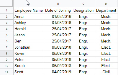
Data in Sheet1 of emp_1:
A1:D contains employee names, dates of joining, designations, and departments.
Data in Sheet2 of emp_2:
A1:E contains the imported data from Sheet1 (employee names, dates of joining, designations, and departments). There is an additional column E for notes, which are manually entered. When more data is added to Sheet1, it will be imported into Sheet2, but I want the notes to remain aligned with the correct employee.
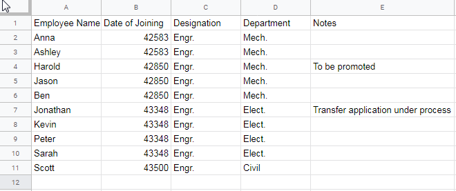
This is what I mean by aligning imported data with manually entered data.
Please note that Sheet2 will be empty initially. We will work on this sheet.
Aligning Imported Data with Manually Entered Data in Google Sheets
To align imported data with manually entered data, you need a unique ID column in both the source sheet and the destination sheet so that we can align them properly.
Google Sheets is a spreadsheet solution that does not automatically generate a unique identifier column for records, unlike a database management system. So let’s manually add the unique ID columns.
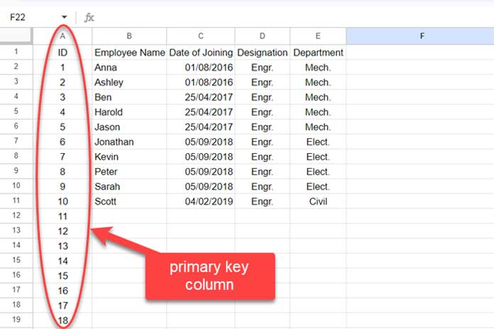
1. Adding a Unique ID (Primary Key) Column in Sheet1
Navigate to Sheet1 of the emp_1 file. Insert a column at the beginning and label it “ID.”
Enter serial numbers (1, 2, 3, …) from A2 to the last row in that column. If you have many rows, you can use the formula =SEQUENCE(ROWS(A2:A)) in cell A2 to fill the column quickly. Then, select the range A2:A, right-click, and choose Copy. Next, right-click again and select Paste Special > Values only.
This step is important because we do not want any formulas in column A.
Optionally, you can enter the following data validation rule for column A to prevent duplicate primary keys from being entered in the future:
- Select the range A1:A.
- Click on Data > Data Validation.
- Select Custom formula under Criteria.
- Enter the following formula:
=COUNTIF(A:A, A1)=1. - Select Reject input under Advanced Options.
Important: If you delete any rows in the future, do not reuse the corresponding ID. For example, if you delete row #2 with ID #1, you should not use ID #1 again thereafter.
2. Adding a Unique ID (Primary Key) Column in Sheet2
Navigate to Sheet2 in emp_2, which is currently an empty sheet.
You can copy and paste the entire column A values from Sheet1 into column A in Sheet2.
These ID columns will serve as the foundation for aligning imported data with manually entered data in Google Sheets.
3. Importing Data and Establishing Relationships between Tables
This third step varies depending on whether you are importing data from two different files (workbooks) or from within the same workbook.
In our case, we are importing data from Sheet1 of emp_1 to Sheet2 of emp_2, so we will use the IMPORTRANGE function.
Enter the following formula in cell B1 of Sheet2:
=ArrayFormula(LET(data, your_import_formula_here, IFNA(VLOOKUP(A1:A, data, SEQUENCE(1, COLUMNS(data)-1, 2), FALSE))))Replace your_import_formula_here with the following IMPORTRANGE formula:
=IMPORTRANGE("enter_emp_1_URL_here", "Sheet1!A1:E")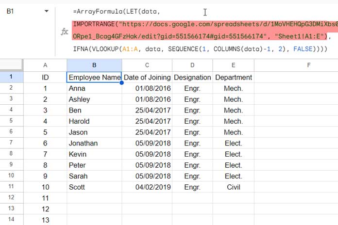
If you are importing data from Sheet1 to Sheet2 within the same file (emp_1), you can simply replace your_import_formula_here with the following formula:
={Sheet1!A:E}Testing the Alignment of Imported Data with Manually Entered Data
We have now connected two tables based on IDs (primary keys).
In Sheet2, enter a few values in column F, such as comments.
Next, navigate to Sheet1 and delete the second row. Check Sheet2, and you will see that the relevant row is empty, indicating that your manually entered data has not shifted.
You can remove the empty rows from Sheet2 as well, ensuring data integrity.
Resources
- Compare Two Tables and Remove Duplicates in Google Sheets
- Combine Two Tables with Unequal Rows Horizontally in Google Sheets
- Merging Two Tables in Google Sheets: The Ultimate Guide
- How to Left Join Two Tables in Google Sheets
- How to Right Join Two Tables in Google Sheets
- How to Inner Join Two Tables in Google Sheets
- How to Full Join Two Tables in Google Sheets
- Master Joins in Google Sheets (Left, Right, Inner, & Full) – Duplicate IDs Solved
- Anti-Join in Google Sheets: Find Unmatched Records Easily
- Combine Two Tables in Excel Using a Dynamic Array Formula


Dear Prashanth,
I followed your training but failed to reach the expected result. Maybe I did something wrong. I have unique ID numbers of trucks with the data on the number of boxes, weight, and volume of each on Sheet1. I use your formula to IMPORTRANGE this data to Sheet2, and I have some adjacent columns to update manually on the same Sheet2 (like a column with comments and some additional information).
Here’s a possible scenario: On Sheet1, truck ID256 and ID258 go one after another, and then after some time, ID257 appears in between, pushing ID258 one row lower. They are reassembled consecutively the same way on Sheet2, and as a result, ID257 gets the comments that refer to ID258, whereas ID258 moves down one row with empty comments. This creates confusion.
It seems that in cases where IDs are reassembled in between, this formula does not work. It only works if you delete or add new rows. Is that so?
Best regards,
Ekaterina
Hi Ekaterina,
A couple of points to make the solution work as expected:
If Sheet1 and Sheet2 are in the same workbook, don’t use IMPORTRANGE. Use FILTER or direct formulas instead to avoid slowing things down.
Keep the ID column in Sheet2 (truck numbers) static. Don’t move them up or down after adding comments. If you need to reorder rows, first copy all values and paste as values, then move the rows (not just IDs), clear unnecessary columns, and reapply the formula.
This way, your comments will stay correctly aligned with the right truck IDs.
Best,
Prashanth
Hi!
Is there a way to remove blank spaces? For example, if I remove the row for “Ben” in Sheet 1, the row for “Ben” will also be removed in Sheet 2. How can I make “Jonathan” and the rest of the rows move up?
Thanks in advance!
Hi Kay,
You can apply a filter to the name column to filter out blank rows. Here are the steps:
1. Select the range of cells that you want to filter.
2. Right-click and select Create a filter.
3. Click on the drop-down arrow in the first cell of the filtered range.
4. Uncheck the Blanks option and click OK.
This will filter out all the rows in the name column that are blank.
I hope this helps! Let me know if you have any other questions.
Hi, Your instructions are helpful.
I’m not very familiar with spreadsheets. But, I used this method to import customer order data. I added a couple of checkboxes and note columns.
Is there a way to sort the data in descending order?
Hi, Tricia,
Use the SORT function in another tab to sort the data as required.
Please see the sample sheet attached:
— URL removed by admin —
Thank you.
Hi, Divya,
Please see the new tab added in your file named “kvp”
Columns:
Light Yellow – manually entered unique IDs.
Light Red – Formula output (Vlookup in cell B2).
Cyan – To manually enter your corresponding data.
Your sheet seems resource-hungry. Remove the last blank columns and rows from all sheet tabs.
Hello Prashanth,
Thank you for such a detailed and clear explanation.
Because I am importing dynamic data using importrange and query to auto-sort to ensure all similar products fall next to each other, the Vlookup to align data is not working.
I will appreciate any help.
Hi, Divya,
Please feel free to share two example sheets in your reply below.
Hello, and thank you for the very useful tutorial.
I followed the above suggestions/guide. The problem is that, in the “end sheet,” the formula returns the data of the “initial” sheet in the first column, not in a row.
Any help would be much appreciated!
Hi, Jason,
It requires a sample sheet to understand and try to solve the problem. You can use two tabs in a single sheet to explain the problem.
Your instructions were very helpful. I now need to do 2 additional things, but am not sure how to integrate that within your formula.
I do wish for the blank rows in the 2nd sheet to disappear if the row was deleted from the 1st sheet.
Also, if someone adds new employees to the bottom of the 1st sheet, I’d like the 2nd sheet to automatically sort by alpha name (which is the column I have the formula in). I’ve used query for this in the past.
Any guidance you can provide would be appreciated!
Hi, Ria g.,
Please go through the below Q&As.
Q) “I do wish for the blank rows in the 2nd sheet to disappear if the row was deleted from the 1st sheet”
A) It’s not possible. Because the ID is still in the second sheet. You may require to use one more sheet (a third sheet) only to filter out the blanks.
In Sheet3, use this Query.
=query(Sheet2!A1:F,"Select * where B is not null",1)But the manual entry must be in Sheet2.
Q) “If someone adds new employees to the bottom of the 1st sheet, I’d like the 2nd sheet to automatically sort by alpha name”
A) To align imported data with manually entered data, we depend on the IDs. So the data will be aligned in the second sheet based on IDs.
To sort by name, let’s depend on Sheet3. Modify the above Query formula in Sheet3.
=query(Sheet2!A1:F,"Select * where B is not null order by B asc",1)Thank you for this tutorial! Is there a way to also apply the Query formula to this? For example, if I want to only import data from the parameters you used when the text in the department column (column E) contains ‘Mech.’??
Hi, Ann,
Updated your Sheets.
I have made the following changes.
1. Inserted an ID column in both the “Source” and “Import” sheets. That is very important to align imported data with manually entered data. Because Google Sheets, not MS Access. It’s a Spreadsheet application.
2. Inserted my formula in B1 in the “Import” sheet.
Now you can proceed to manual entry in other columns in “Import”.
Later use the set Filter in B1 to filter out blanks.
Hello! Thanks a lot for this tutorial! this method helped however my issue now is that if I add more rows in between some existing rows in EMP 1, it does not reflect on EMP 2. Is there any way I’m able to do this? Thank you!
Hi, sxn,
Please see my answer above to Jacques Granjon.
Hi Prashanth, and thanks a lot for your detailed tutorial.
I followed it step by step and adapted it to my needs, however, I’m still facing an issue.
I need to add new rows between already existing rows, let’s say 3 rows between lines 7 and 8 on EMP1. For sure on EMP1 that’s working fine, but it does not automatically add a row at the very same place on EMP 2, between lines 7 and 8. Is there maybe a way to do this?
Thanks in advance,
JA
Hi, Jacques Granjon,
It all depends on how you present the unique IDs in EMP 2.
If you want to make EMP 2 data in the same order in EMP 1, you may require a new tab in EMP 2.
In that new tab, in the first column, import the IDs from EMP 1.
In the second column, Vlookup the imported IDs (use the imported IDs as the search keys) with the data in the first tab in EMP 2.
Here is an example sheet.
Example_30121
In this, please delete the values in column D in “Tab A” as it’s written for another user.
In that read TAB A as IMP 1 and TAB B as IMP 2. TAB C is just for aligning TAB B data with TAB A data. It has no other use.
I had tried your method but the problem is, my data are automatically updated in the top row.
In my project, I connect my master sheet with another application through API. Then again connect the master G Sheet with another sheet(Sheet B) to display certain columns only.
Now I placed the unique IDs in Sheet B and Sheet C to have a connection.
But the problem is my data in the master sheet are updated in the first row which makes other sheets update data in the first row…How can I solve this problem??
Hello, My name is Rita.
I did exactly what you posted, but the result is not the same.
As if the EMP2 B2 matches the EMP1 B2, but the EMP2 B3 matches the EMP1 C3, the EMP2 C4 matches the EMP1 D4 and then nothing more appears. What am I doing wrong?
Thank you
Rita Macedo
Hi, Rita Macedo,
To find the reason, I maybe wanted to see what’s happening on your side. For free assistance, you can share the link to that files in your reply to this thread (the links won’t be published).
Hi – Thanks for this. As always, your tutorials and knowledge are exemplary!
I’ve tried to use your solution in building an ‘Inbox Follow Up’ system that I am designing. As your tutorial detailed, I needed to be able to keep my follow up actions linked to a daily updated inbox which was being imported via a .CSV.
The problem is: I need to display the information ‘like an inbox’, i.e sorted by date order with the newest message at the top. The solution you have provided maps dynamic data to static data, however, I believe that I need it to be the other way around (static to the dynamic), or have the means to sort the entire sheet once the dynamic has loaded in.
Can you please advise if your solution could be adapted to achieve this, or are there other approaches you’d recommend, or do I need to look at a scripted method?
Many thanks,
Dale.
Hi, Dale,
Can you explain it with a live example sheet? Feel free to share the sheet link in the comments (won’t be published).
For those still searching for a way to keep data query and manual entries aligned in MICROSOFT EXCEL.
YouTube link.