There is a misconception that the Indirect function can be used to get dynamic sheet names in Importrange.
Many users try using the Indirect function as the range_string in Importrange and get an error. Then what is the solution? Read on to find out.
Let’s begin with the use of the Importrange function in Google Sheets. The Importrange function is actually used to import data from one Spreadsheet sheet to another Spreadsheet.
It has one advantage over traditional copy and paste: when you update your source data, the imported data will also be updated.
What Are Dynamic Sheet Names in the Importrange Function in Google Sheets?
You can understand this with a simple example.
Suppose you have one Google Sheets workbook with three sheets and the tabs named “Jan”, “Feb”, and “Mar”. You want to selectively import data from these sheets to another Google Sheets workbook.

See how I am controlling the sheet names in the Importrange function. I can use a dropdown to select the sheet to import the data from the source workbook.
My Importrange formula is in cell B1. Based on the selected option in the dropdown menu (the sheet name), the formula dynamically imports data from different sheets in the workbook!
How to Get Dynamic Sheet Names in Importrange in Google Sheets
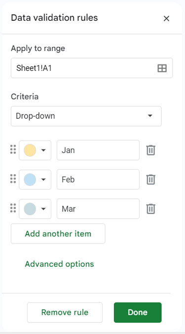
To get dynamic sheet names in the Importrange function, the first step is to create a Data validation dropdown menu containing the sheet names to import.
Here, I have my dropdown menu in cell A1. It was created through the Insert menu > Drop-down as shown below.
Must Try: Multi-Row Dynamic Dependent Drop-Down List in Google Sheets.
Now, let’s take a look at the Importrange function syntax. We are playing with the range_string argument in the formula.
IMPORTRANGE(spreadsheet_url, range_string)Now, see my dynamic Importrange formula in cell B1.
=IMPORTRANGE("enter_spreadsheet_url_here",A1&"!A1:C")Note: Please don’t forget to replace enter_spreadsheet_url_here with the workbook URL.
In this formula, the sheet name (tab name) is only dynamic. The import range reference is set to A1:C.
If you want to bring more dynamism to this formula, I mean to control the range too, create another dropdown.
To do this, you should first create Named ranges in the source file. You can learn the tips below.
Dynamic Sheets Names and Range in Importrange
Steps:
Go to your source file and in each sheet tab, create Named ranges. Naming a range means, as it suggests, giving a name to a range of cells.
As I mentioned earlier, I have three sheet tabs. In the first sheet tab (Jan), I am creating a named range for the range A1:C.
I have selected the range A1:C. Now, I want to click on the Data menu > Named ranges. I am naming this range as table1.

Then, go to the second sheet tab (Feb). Select the range that you want to import and name the range as table2.
Continue this in the third sheet tab (Mar) and name the range as table3. Once complete, come back to the sheet where we have our dropdown and the Importrange formula entered.
Create one more dropdown in cell A2 containing the above-named ranges as the dropdown list.
Now, you should modify our earlier formula.

See the new modified formula.
=IMPORTRANGE("enter_spreadsheet_url_here",A1&"!"&A2)This formula is responsive to both sheet names and ranges.
That’s all! This is how you can bring dynamism to the Importrange function in Google Sheets.


Omggg
Thank you very much for this topic. I was searching for this everywhere on google.
In my requirement, I need to use a single formula to fetch values from file B across all sheets. Here I couldn’t use dropdown bcoz I need to see data from all 3 sheets at a time.
I mean 1st row may have data from sheet ‘Jan’. 2nd row may have data from ‘Feb’ and so. Is there any solution for this?
Kindly help. Thanks in advance
I forgot to mention that I am using Vlookup function to fetch data from File B based on unique code, code for each item in Jan, Feb, Mar sheets.
I am using the Importrange function inside Vlookup.
Hi, Divya,
Please wait for my next tutorial. A similar tutorial is already in the pipeline. In that, I won’t write the Vlookup part since it’s already explained.
1. Align Imported Data with Manually Entered Data in Google Sheets.
2. How to Vlookup Importrange in Google Sheets [Formula Examples].