In Excel, the XLOOKUP function isn’t inherently designed to exclusively work with visible rows; you’ll need a workaround for this. One common approach in Excel involves using the FILTER function within the XLOOKUP’s lookup_array and result_array parameters.
However, this method doesn’t directly address the issue of identifying visible and hidden rows in Excel. Consequently, changes made to the filter in the Excel table won’t be reflected in the XLOOKUP results unless you modify the FILTER function accordingly.
To correctly use XLOOKUP with visible rows in Excel, you’ll need to employ a different strategy. For educational purposes, I’ll also demonstrate using the FILTER function.
Sample Data and Regular XLOOKUP
In my Excel spreadsheet, I have sample data consisting of Product, Category, Price, and Stock, located in cell range A1:D10, where A1:D1 contains the labels.
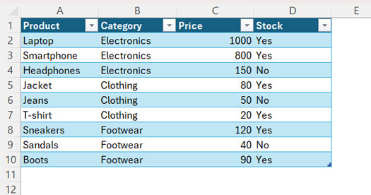
The last column, Stock, indicates whether a product is available with “Yes” or “No”.
To look up a product in column A, such as “Jeans”, and return its price from column C, we can use the following XLOOKUP formula in Excel:
=XLOOKUP("Jeans", A2:A10, C2:C10)Note: You’re also free to input “Jeans” into a cell and use that cell reference instead.
In this formula, “Jeans” is the lookup_value, A2:A10 is the lookup_array, and C2:C10 is the return_array, following the syntax of XLOOKUP in Excel:
=XLOOKUP(lookup_value, lookup_array, return_array, [if_not_found], [match_mode], [search_mode])This formula will return the price of $50.
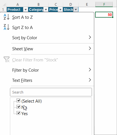
Now, let’s filter out rows where column D contains “No”. To do this, click on the drop-down arrow in cell D1, uncheck “No”, and click “OK”.
Despite filtering, the result remains the same. However, how can we ensure that hidden rows are omitted from the XLOOKUP result in the Excel spreadsheet?
XLOOKUP in Visible Rows in Excel: The Proper Way
To exclude hidden rows in Excel using XLOOKUP, we’ll manipulate the lookup_array through a workaround.
We’ll remove values in hidden rows from this array so that XLOOKUP fails to match the lookup_value in the lookup_array.
How do we achieve this in Excel?
We’ll use a formula, let’s call it hidden_row_identifier_formula, in the following syntax to manipulate A2:A10.
Generic Formula:
=XLOOKUP(lookup_value, IF(hidden_row_identifier=1, lookup_array, ""), return_array)In this, the hidden_row_identifier can be either of the following:
MAP(lookup_array, LAMBDA(r, SUBTOTAL(103, r)))
SUBTOTAL(103, OFFSET(first_cell, ROW(lookup_array)-ROW(first_cell), 0))
Yes, there are two formulas: one using a MAP Lambda function and one without.
Here’s an example of using XLOOKUP in visible rows in Excel:
=XLOOKUP("Jeans", IF(MAP(A2:A10, LAMBDA(r, SUBTOTAL(103, r)))=1, A2:A10, ""), C2:C10)Where:
lookup_value: “Jeans”lookup_array:IF(MAP(A2:A10, LAMBDA(r, SUBTOTAL(103, r)))=1, A2:A10, "")return_array: C2:C10
The lookup_array can also be: IF(SUBTOTAL(103, OFFSET(A2, ROW(A2:A10)-ROW(A2), 0))=1, A2:A10, "")
Breakdown of Formula (hidden_row_identifier_formula)
There are two parts:
Part #1: MAP(A2:A10, LAMBDA(r, SUBTOTAL(103, r))) or SUBTOTAL(103, OFFSET(A2, ROW(A2:A10)-ROW(A2), 0))
The formula =SUBTOTAL(103, A2) returns 1 if cell A2 contains any value and 0 otherwise. This function behaves similarly to the COUNTA function but excludes hidden cells.
Our objective is to apply this formula to each row in the lookup_array, specifically A2:A10. To achieve this, we have utilized the MAP lambda function in one approach and the OFFSET function in another approach.
Part #2: IF(part_1=1, A2:A10, "")
This formula returns values in A2:A10 wherever part_1 returns 1, otherwise it returns blank.
Note: I recommend using the OFFSET function instead of Lambda in Excel for better performance, particularly when working with large datasets.
XLOOKUP with FILTER Function in Excel
Excel offers the FILTER function to selectively filter a range or table based on specified conditions.
Syntax: FILTER(array, include, [if_empty])
In the example provided, if you want to search column A for an item and return its price from column C only if column D indicates “Yes”, you can achieve this using a combination of XLOOKUP and FILTER.
=XLOOKUP("Jeans",FILTER(A2:A10,D2:D10="Yes"),FILTER(C2:C10,D2:D10="Yes"))Where:
lookup_value: “Jeans”lookup_array:FILTER(A2:A10, D2:D10="Yes")return_array:FILTER(C2:C10, D2:D10="Yes")
It’s important to note that this approach does not directly replicate the functionality of XLOOKUP with visible rows. Instead, it involves using XLOOKUP after filtering out rows based on specified conditions.


