Filtering data from the previous month may be useful for comparative analysis, generating reports, problem identification, forecasting, etc.
This tutorial explains how to use the FILTER function to filter data from the previous month in Excel for Microsoft 365.
If you are currently using something like this formula: =FILTER(filter_range, MONTH(date_column) = MONTH(TODAY())-1), I recommend against it.
While it might return the correct result at present, it will fail in two scenarios:
- It will fail when the current month is January because
MONTH(TODAY())-1will result in 0, instead of 12 in January. - If your data spreads across two or more years, the formula may filter data from multiple years as the year part is not used in the criterion.
The proper formula to filter data from the previous month in Excel is:
=FILTER(
   filter_range, MAP(date_column,
   LAMBDA(r, EOMONTH(r, -1)+1)) = EOMONTH(TODAY(), -2)+1
)
When using this formula:
After filtering, the date column in the result will return as date values. To format them, select the column and choose a desired date format (e.g., “Short Date”) from the Number group on the Home tab.
Example: Filter Previous Month’s Data in Excel
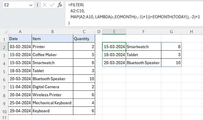
The sample data range is A1:C10, where column A contains dates, column B contains item names, and column C contains quantities.
We will filter the range A2:C10, excluding the header row A1:C1, as it contains field labels. Including the header row in the filter range may cause the formula to fail because it employs a date criterion.
Before proceeding with the sample data, it’s important to note that the current month is April 2024. Therefore, the formula will filter the data from March 2024.
However, when using this formula, it’s essential to understand that it will take the current month from the date you use the formula (based on your system clock date on that day).
Formula:
=FILTER(
   A2:C10,
   MAP(A2:A10, LAMBDA(r, EOMONTH(r,-1)+1))=EOMONTH(TODAY(), -2)+1
)
Where A2:C10 is the filter_range and A2:A10 is the date_column range. Don’t forget to apply “Short Date” formatting to the date column range in the result.
The above demonstrates the correct method for filtering data from the previous month using a formula in Excel.
Formula Breakdown
Before delving into the explanation of the formula, let me address a limitation I’ve encountered with dynamic array formulas in Excel.
Unfortunately, dynamic array formulas are not capable of spilling all date functions. For instance, while the formula =MONTH(A2:A10) will return the month numbers from A2:A10, it won’t spill EOMONTH(A2:A10, 0).
With that in mind, let’s examine how the formula filters the previous month’s data.
Syntax:
FILTER(array, include, [if_empty])Where:
array: A2:C10include:MAP(A2:A10, LAMBDA(r, EOMONTH(r,-1)+1))=EOMONTH(TODAY(), -2)+1
The crucial aspect of filtering by the previous month lies in the ‘include’ part. Let’s delve deeper into it.
MAP(A2:A10, LAMBDA(r, EOMONTH(r, -1)+1)): This segment converts the dates in A2:A10 to the beginning of the month dates. Since EOMONTH doesn’t spill on its own in Excel, we utilize the MAP lambda function to iterate through each row in the range A2:A10 within EOMONTH.EOMONTH(TODAY(), -2)+1: This expression returns the beginning of the month date of the previous month.
The formula filters A2:C10 if the beginning of the month dates in A2:A10 are equal to the beginning of the month date in the previous month.
This approach is the correct method to filter the previous month’s data from a table in Excel.
The advantage lies in using a date as the criterion rather than a month number. Using a month number can lead to issues, especially when the current month is January (1), as subtracting 1 would result in 0, not 12.


