Using Power Query and a Dynamic Array Formula, you can efficiently unpivot cross-tabular formatted data into a more manageable tabular format in Excel.

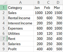
Cross-Tabular Format: Cross-tabular data resembles a grid where each row signifies a category (e.g., cash flow account heads), and each column represents another category (e.g., months). The cell values depict the corresponding values for each combination of categories, such as the cash flow amount for an account head in a specific month.

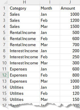
Tabular Format: Tabular data is organized in rows and columns, like a typical table. Each row is a separate record, and each column represents a different aspect of those records (like category, month, and cash flow amount). This format makes it easy to see individual data points and analyze them.

To transform cross-tabular data into a tabular format for easier manipulation and analysis, we can use Excel tools like Power Query or Dynamic Array Formulas. These methods help quickly convert the data, making it more manageable for further analysis.

Unpivot Data Using a Dynamic Array Formula in Excel

The dynamic formula utilizes Excel functions such as IFERROR, TEXTSPLIT, LET, VSTACK, TOCOL, HSTACK, and REDUCE to unpivot data.

You don’t need to be familiar with these functions to unpivot your data in Excel. You can try this formula if your Excel version supports it (currently available in Microsoft 365). Otherwise, you can proceed with the Power Query approach.

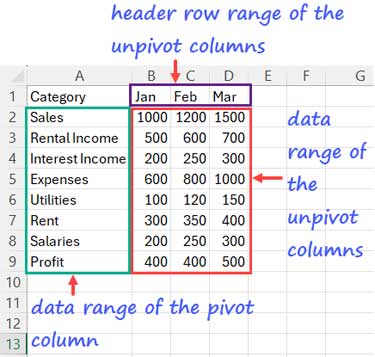
In the formula, one needs to correctly specify the data range of the pivot column, the header row range of the unpivot columns, and the data range of the unpivot columns.

In our example, the pivot column’s data range is A2:A9, the header row range of the unpivot columns is B1:D1, and the data range of the unpivot columns is B2:D9.

Insert the following formula in cell H1 to transform the cross-tabular data into tabular data, also known as unpivoting the data (please refer to the second screenshot from the top to see the output).

=REDUCE(
   HSTACK("Title1", "Title2", "Title3"), 
   TOCOL(A2:A9&"|"&B1:D1&"|"&B2:D9), 
   LAMBDA(a, v, VSTACK(a, LET(ts, TEXTSPLIT(v, "|"), IFERROR(ts*1, ts))))
)

Note: Replace “Title1”, “Title2”, and “Title3” in the formula with your desired field labels for the new unpivoted data table.

Formula Explanation

Syntax: REDUCE([initial_value], array, lambda(accumulator, value))

The REDUCE function in Excel reduces an array by applying a lambda function to each value in it, row by row. Each application produces an intermediate value, which accumulates in an accumulator. The formula returns the final result contained in the accumulator.

• initial_value: HSTACK("Title1", "Title2", "Title3") – row header labels for the unpivoted data.
• array: TOCOL(A2:A9&"|"&B1:D1&"|"&B2:D9) – combines the pivot data range, unpivot data headers, and unpivot data range into a column.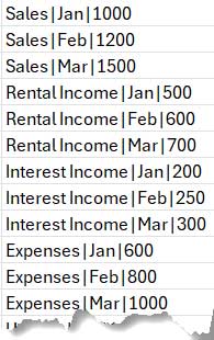
  
• accumulator: ‘a’ – the initial value in the accumulator is the title for unpivoted data (HSTACK("Title1", "Title2", "Title3")).
• value: ‘v’ – represents each value in the array.

The formula expression within the Lambda:

• VSTACK(a, LET(ts, TEXTSPLIT(v, "|"), IFERROR(ts*1, ts)))

‘v’ represents the first row in the array. TEXTSPLIT splits it based on the “|” delimiter. LET function names this expression ‘ts’.

IFERROR multiplies ‘ts’ by 1 and returns ‘ts’ if it’s non-numeric. Otherwise, it returns ‘ts*1’. This step addresses the issue where TEXTSPLIT converts numeric or date data types to text.

VSTACK function stacks the initial value (the header row of the unpivoted table) with this output.

The REDUCE function repeats this process for each row.

This logic underlies the dynamic array formula that unpivots data in Excel.

Unpivot Data Using Power Query in Excel

Follow these step-by-step instructions to unpivot data using Power Query in Excel:

1. Start by selecting any cell within your data, such as cell A1 (A1:D9 is our sample data range to unpivot).
2. Navigate to the Data menu and click on the ‘From Table/Range’ icon in the Get & Transform Data group. If it prompts you with a ‘Create Table’ dialog box, click OK.
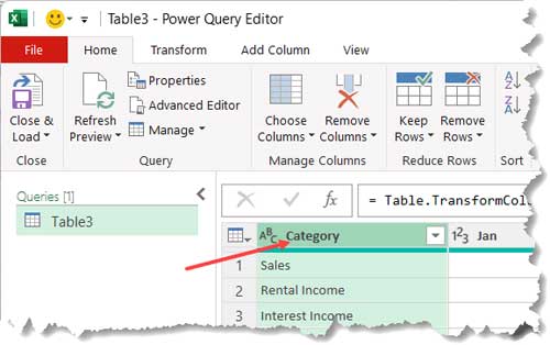
3. In the Power Query Editor that appears, locate your table. Right-click on the field label of the column you don’t want to unpivot, such as “Category,” and choose “Unpivot Other Columns.”
   
4. Excel will swiftly unpivot the data within the Power Query editor.
5. To load the unpivoted data back into your Excel spreadsheet, click the ‘Close & Load’ command on the Home tab of the Power Query editor.
   
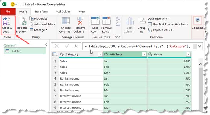
6. Excel will load the unpivoted data into a new worksheet tab of your spreadsheet.

Conclusion

We have explored two options for unpivoting data in Excel. Which one should you choose?

Dynamic Array Formula:

• Provides a more direct approach within the Excel environment.
• Offers flexibility in terms of data manipulation, allowing for customization according to specific requirements.
• Suitable for users who prefer working with formulas.

Power Query:

• Offers a user-friendly interface for data transformation tasks.
• Supports more complex data transformation operations beyond simple unpivoting.

Depending on the specific requirements of the task and the user’s familiarity with Excel functions and tools, one may choose either the Dynamic Array Formula or Power Query for unpivoting data.