There is a built-in function for counting distinct values in a Google Sheets Pivot table, which is COUNTUNIQUE.
However, for the unique count of values in the Pivot table, you may need to rely on a helper column in the source data with the top row containing an array formula.
Understanding “Distinct” and “Unique”
Before we delve into these methods, let’s understand the difference between “distinct” and “unique,” as these terms are often used interchangeably.
In the following table, there are 4 distinct names and 3 unique names:
| Name | Distinct | Unique |
| Ann | Yes | |
| Jasmine | Yes | Yes |
| Roy | Yes | Yes |
| Ann | ||
| Joshua | Yes | Yes |
The name “Ann” appears twice. When counting distinct names, we will consider this as 1, whereas when counting unique names, we will not consider duplicates.
This guide belongs to the Pivot Table Calculations & Advanced Metrics hub—your reference for advanced pivot table calculations in Google Sheets.
Counting Distinct Values in Pivot Table
Let’s consider a sample sales report in the range A1:C21 in Sheet1 of Google Sheets, containing columns for area (category), name (employee names), and item (product).
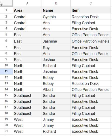
Unnecessary columns like dates have been removed to avoid clutter.
You can make a copy of the sample sheet below, which will help you follow this tutorial step by step.
How do we get the distinct count of employees in each area?
Creating the Pivot Table:
- Select the range A1:C21.
- Click on Insert > Pivot table.
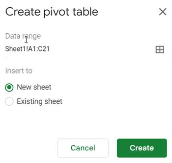
- In the window that appears, ensure the range is set to Sheet1!A1:C21 and select “New sheet” for the inserted pivot table.
- Click Create.
Google Sheets will add a new sheet containing a blank report layout.
Adding Fields to the Layout:
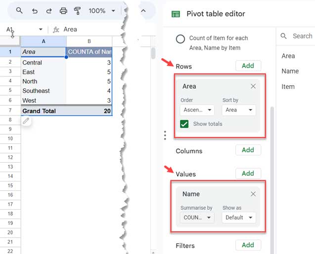
We aim to calculate the distinct count of employees by area in the Pivot table. To achieve this:
- Drag and drop the ‘Area’ field under “Rows.”
- Drag and drop the ‘Name’ field under “Values,” as we need to count these values.
Once you’ve completed these steps, the Pivot table report will be populated with the employee count for each area.
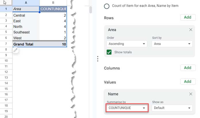
Getting the Distinct Count in the Pivot Table:
In the Pivot table values field, select the COUNTUNIQUE function. That’s all.
Counting Unique Values in Pivot Table
In the above example, we obtained the count of distinct employees (names) in each area using the Pivot table.
However, what if we want to count employees (names) in each area but exclude them from the count if they are engaged in more than one area? Such counting will help you manage your manpower efficiently.
Unfortunately, there is no specific function within the Google Sheets Pivot table for this. Instead, you need to depend on a helper column.
Helper Column:
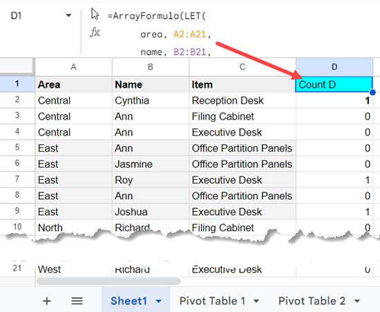
Insert the following formula in cell D1. This formula will populate D2:D21 with the values 0 or 1.
=ArrayFormula(LET(
      area, A2:A21,
      name, B2:B21,
      rc,
         COUNTIFS(
            area&name, area&name, ROW(area), "<="&ROW(area)
         ),
      VSTACK(
        "Count D",
         IF(COUNTIFS(IF(rc=1, name, ""), IF(rc=1, name, ""))=1, 1, 0)
      )
))
Where:
- A2:A21 represents the area (category) reference.
- B2:B21 represents the name reference, which is the column for the unique count.
Wherever the formula returns 1, it indicates a unique deployment of an employee in that area.
Pivot Table Settings for Unique Count:
To force the Pivot table to return a unique count instead of a distinct count, make three changes:
- When creating the Pivot table, select the range A1:D21.
- Drag and drop the “Count D” (helper column) field below values instead of “Name.”
- Select SUM instead of COUNTUNIQUE.


