In Excel, the easiest way to sum values in a range by categories is by using the UNIQUE and SUMIF functions.
If you’re using Excel in Microsoft 365, just two dynamic array formulas can summarize a large dataset. We’ll explore both options: the regular method and the dynamic array method.
The sample data consists of office expenses. The dates of expenses incurred are in column A, the descriptions of the expenses are in column B, and the amounts incurred are in column C.
The data range is A1:C15, where A1:C1 is the header row, so we won’t include that row in the calculations.
Therefore, we need to extract the unique categories in B2:B15 and sum the corresponding amounts in C2:C15.
Step By Step Instructions
Please follow the step-by-step instructions below to sum values by categories in an Excel spreadsheet.
- Enter the following formula in cell E2 to get the unique categories from B2:B15:
=UNIQUE(B2:B15)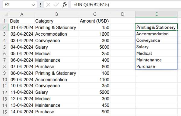
- In cell F2, enter the following SUMIF formula to return the sum of the first category:
=SUMIF($B$2:$B$15, E2, $C$2:$C$15)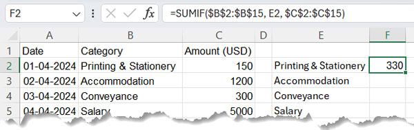
This formula follows the syntaxSUMIF(range, criteria, sum_range), where:range: $B$2:$B$15 (category range)criteria: E2 (the first category in the unique list)sum_range: $C$2:$C$15
We made therangeandsum_rangereferences absolute (see the dollar signs) as we don’t want them to change when we copy-paste it for other criteria in the unique list.
- Click the fill handle in cell F2 and drag it down as far as you want, until the last row in the UNIQUE result.
Sum Values by Categories Using a Dynamic Array Formula in Excel
It’s luckier if you are using Excel in Microsoft 365. You won’t need to drag the SUMIF formula down.
You can skip the third step in the regular approach mentioned above for summing values by category.
Instead, you can replace the previous SUMIF formula in cell F2 with the following:
=SUMIF(B2:B15, E2#, C2:C15)This means you need two formulas: one UNIQUE in cell E2 and one SUMIF in cell F2, to sum values by categories in Excel.
Further Enhancements
Do you need a single formula to sum values by categories in Excel for Microsoft 365? Follow the steps below:
Let’s start fresh.
- In cell E2, enter the following formula to get the sum of values by categories:
=SUMIF(B2:B15, UNIQUE(B2:B15), C2:C15)
where:range: B2:B15 (we don’t need to specify an absolute reference since we are not going to copy-paste the formula down as before)criteria: UNIQUE(B2:B15)sum_range: C2:C15 (absolute reference is not required compared to the earlier formula)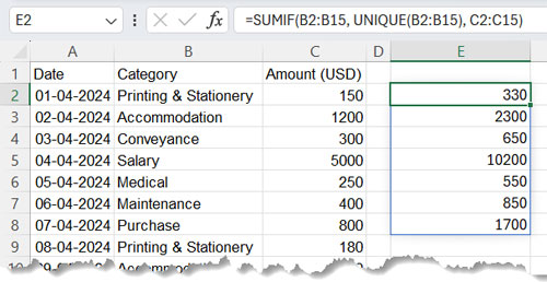
- Stack the unique categories onto this output. For that, we can use the HSTACK function as follows:
=HSTACK(UNIQUE(B2:B15),SUMIF(B2:B15,UNIQUE(B2:B15),C2:C15))- The syntax is:
HSTACK(array1, array2) - where
array1is the UNIQUE formula andarray2is the SUMIF formula.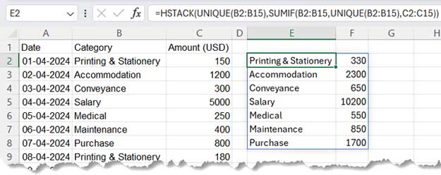
- The syntax is:
- We can improve the performance of this formula by removing the repeated calculation of UNIQUE. Use LET to name the unique formula as follows:
=LET(categories,UNIQUE(B2:B15),HSTACK(categories,SUMIF(B2:B15,categories,C2:C15)))
This dynamic array formula sums values in a range by categories in Excel.
Resources
Here are a few related resources for Excel.


