Suppose you prefer to sum by month in Excel using a formula. In that case, you can consider three approaches: a basic helper column-based formula, a dynamic array formula, and a custom reusable function.
This tutorial covers all the options, allowing you to choose the one based on your requirements. Remember, while all options are simple, the learning curve may vary depending on your skill level.
Helper Column-Based Formula: Ideal for those comfortable using helper columns and multiple formulas for each month.
Dynamic Array Formula for Sum by Month: The user needs to specify the references for the date and amount columns. The formula then generates the summary report for all the months at once.
Custom Reusable Function: Derived from the dynamic array formula, this function is beneficial if you use the same formula with multiple datasets in the workbook. It employs an easy-to-remember name.
Sample Data Setup for Formula Examples
We have the following sample data in cells A1:B10 in an Excel spreadsheet:
| Date | Amount |
| 31-12-2023 | 1000 |
| 31-12-2023 | 500 |
| 14-04-2024 | 2000 |
| 26-05-2024 | 1500 |
| 26-05-2024 | 2500 |
| 27-05-2024 | 1750 |
| 01-06-2024 | 250 |
| 01-06-2024 | 3000 |
| 15-06-2024 | 0 |
This sample data includes dates spanning four months (December 2023, April 2024, May 2024, and June 2024) along with corresponding amounts.
Let’s apply sum-by-month formulas to this sample data in Excel.
Basic SUMIFS Formula for Sum by Month in Excel
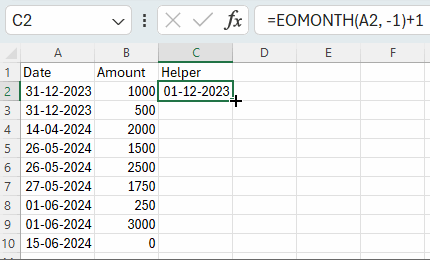
This is the helper column approach. So let’s prepare the helper column first.
In cell C1, optionally, enter the label “Helper”. This will help in the future to recognize the purpose of the column.
In cell C2, enter the following formula:
=EOMONTH(A2, -1)+1This will return the beginning of the month date of the date in cell A2.
Navigate to cell C2, if not already there, click the fill handle (square in the bottom right corner) and drag it down to the cells where you want to copy the formula.
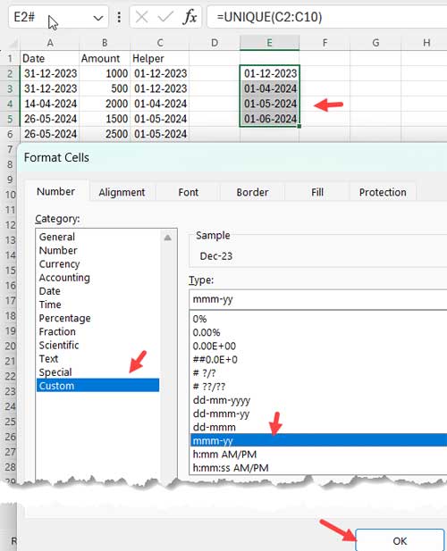
Then insert the following UNIQUE formula in cell E2 to generate the unique beginning of the month dates in E2:E5.
=UNIQUE(C2:C10)Select cells E2:E5.
Under the Home tab, click the drop-down within the Number group and select More Number Formats. This will open the Format Cells dialog box in Excel.
Click Custom, select mmm-yy under the “Type” and click OK.
In cell F2, enter the following SUMIF formula:
=SUMIF($C$2:$C$10, E2, $B$2:$B$10)Where; C2:C10 is the range, E2 is the criterion, and B2:B10 is the range to sum.
Drag the fill handle of cell F2 down.
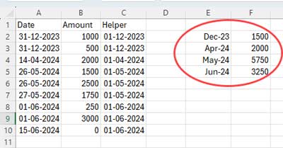
That’s summing by month using the helper column approach in Excel.
Dynamic Array Formula for Sum By Month in Excel
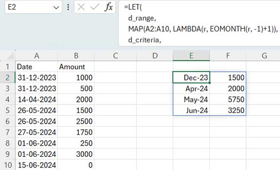
If you are using Excel in Microsoft 365, you can use the following dynamic array formula to sum by month:
=LET(
   d_range,
   MAP(A2:A10, LAMBDA(r, EOMONTH(r, -1)+1)),
   d_criteria,
   UNIQUE(d_range),
   amt, B2:B10,
   HSTACK(
      d_criteria,
      MAP(d_criteria, LAMBDA(r, SUMPRODUCT((d_range=r)*amt)))
   )
)
Enter this formula in cell E2.
Select E2:E5 and apply mmm-yy formatting as per our previous helper formula-based approach.
Note: If any cell is blank in the A2:A10 range, the formula result will contain errors.
How do I use this formula with a different data range in my Excel spreadsheet?
In this sum-by-month dynamic array formula, A2:A10 refers to the date range and B2:B10 refers to the amount range. You replace them with your corresponding range references.
Formula Explanation
Syntax:
=LET(name1, name_value1, name2, name_value2, name3, name_value3, calculation)Where:
MAP(A2:A10, LAMBDA(r, EOMONTH(r, -1)+1)): Returns beginning of the month dates in A2:A10. This isname_value1, and the assigned name isd_range(name1).UNIQUE(d_range): Returns the unique beginning of the month dates. This isname_value2, and the assigned name isd_criteria(name2).- B2:B10: The amount column reference. This is
name_value3, and the assigned name isamt(name3).
Sum by Month Calculation (it uses the assigned names and values):
HSTACK(
      d_criteria,
      MAP(d_criteria, LAMBDA(r, SUMPRODUCT((d_range=r)*amt)))
   )
The key part of this calculation is the following SUMPRODUCT formula:
SUMPRODUCT((d_range=r)*amt)Explanation:
d_range=r: In this,d_rangeis the beginning of the month date range, andris the first value in thed_criteria.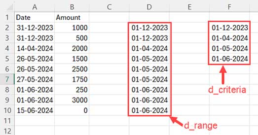
- This means it checks whether the first value in the
d_criteriais equal to any value ind_range, returning an array with TRUE (1) or FALSE (0).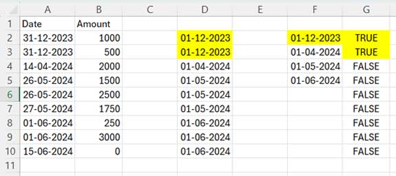
- Multiplying that with the amount
amt[(d_range=r)*amt] returns an array where TRUE corresponds to the amount and FALSE corresponds to 0. - SUMPRODUCT returns the sum of this array, giving the total amount corresponding to the first criterion in the
d_criteria. - The MAP function iterates over each value in
d_criteriaand produces the month-wise summary amount. - The HSTACK function stacks the
d_criteriawith this result, forming the month-wise summary report.
Custom SUMBYMONTH Function for Reusable Sum By Month Calculations
We can convert the sum-by-month dynamic array formula into a reusable function within a workbook.
This is a relatively straightforward approach since we already have the formula. Let’s name the function SUMBYMONTH() and define it as follows.
We need to replace the range A2:A10 and B2:B10 in the dynamic array formula with the parameters we want to use within the SUMBYMONTH() custom function.
Steps
To do this, we use the LAMBDA function in the following syntax:
=LAMBDA(parameter1, parameter2, calculation)Let’s specify ‘range’ as parameter1 and ‘sum_range’ as parameter2. The calculation will be the sum-by-month dynamic array formula. But in that, you should replace A2:A10 with ‘range’ and B2:B10 with ‘sum_range’. Here it is:
=LAMBDA(range,sum_range, LET(d_range,MAP(range,LAMBDA(r,EOMONTH(r,-1)+1)),d_criteria,UNIQUE(d_range),amt,sum_range,HSTACK(d_criteria,MAP(d_criteria,LAMBDA(r,SUMPRODUCT((d_range=r)*amt))))))To create the custom function, copy this formula and open the workbook in which you want to use it.
- Go to the Formulas tab.
- Click Name Manager within the Defined Names group.
- In the Name Manager dialog box, click New.
- Type the name SUMBYMONTH in the Name field.
- Select Workbook within the Scope field.
- In the Refer to field, replace the existing reference with the copied formula.
- Click OK and Close the Name Manager dialog box.
You are now set to use the SUMBYMONTH() named function and the syntax is:
=SUMBYMONTH(range, sum_range)In our example, you can use the following formula to dynamically return a month-wise summary report:
=SUMBYBOMTH(A2:A10, B2:B10)Don’t forget to format the first column of the result to mmm-yy. Also, make sure that there are no empty cells in the date range, here A2:A10.


