I believe comparing the differences in how the FILTER functions work in Excel and Google Sheets is important. While they both do the same basic thing, they have some differences.

Google Sheets has had the FILTER function for a while now, but in Excel, it’s part of a newer feature called Dynamic Arrays, which is available in Microsoft 365.

If you’re used to using Excel and switch to Sheets, you might not have much trouble with the FILTER function, except for one thing: in Excel, you might need to add an extra bit of information.

But if you’re used to Google Sheets and start using Excel, you might find it tricky sometimes.

So comparing how the FILTER function works in Excel and Google Sheets can help you understand these differences.

FILTER Function Argument Comparison

Syntax in Google Sheets:

FILTER(range, condition1, [condition2, …])

Syntax in Excel:

FILTER(array, include, [if_empty])

The difference is evident from the syntax itself.

1. Range to Filter:
   range (Google Sheets) – refers to the range of data to filter, which can be single-dimensional or two-dimensional.
   array (Excel) – equivalent to range in Google Sheets.
2. Criteria Specification:
   condition1, [condition2, …] (Google Sheets) – condition1 represents a row or column evaluating TRUE or FALSE, or containing TRUE or FALSE values. Additional conditions (condition2, …) can be added.
   include (Excel) – similar to condition1 in Google Sheets, representing a row or column, evaluating TRUE or FALSE, or containing TRUE or FALSE values.
3. No Match:
   If_empty (Excel) – Value to return when no results are returned.

Google Sheets allows specifying multiple conditions (condition1, [condition2, …]) individually, whereas Excel doesn’t (include).

So, how do we specify multiple conditions in the FILTER function in Excel?

We will delve into that in the comparison part below.

How the FILTER Functions Differ in Excel and Google Sheets

The FILTER formulas in Excel will function properly in Google Sheets as long as you don’t include the last argument, if_empty, in the formula. However, some variations of the Google Sheets FILTER formulas won’t work in Excel.

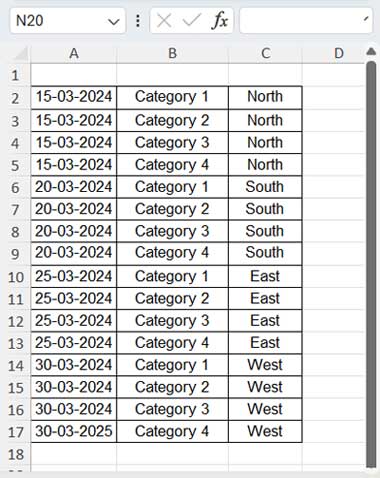
Let’s use a sample dataset for comparing the FILTER function in Excel and Google Sheets. The data includes dates in column A, categories in column B, and regions in column C, with the range being A2:C17.

Handling No Match Errors: Tallying Arguments

The following formula will return #CALC! in Excel and #N/A! in Google Sheets:

=FILTER(A2:C17, B2:B17="Category 5")

This occurs because B2:B17="Category 5" returns an array of FALSE values when there is no match in B2:B17.

To address this error in Excel, you can replace it with custom text as follows:

=FILTER(A2:C17, B2:B17="Category 5", "Not Found!")

However, in Google Sheets, you can use the IFNA function to wrap the formula, like this:

=IFNA(FILTER(A2:C17, B2:B17="Category 5"), "Not Found!")

Filter Function in Excel vs. Filter Function in Google Sheets: Dealing with Multiple Criteria

OR Criteria (Matching Either of the Criteria):

When filtering with OR criteria, there is no difference in using the FILTER function in Excel and Google Sheets.

To extract “Category 1” or “Category 2” from the range or array, we can use the following formula in both Excel and Google Sheets:

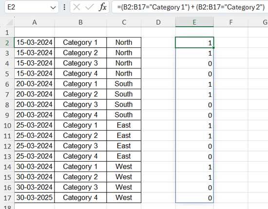
=FILTER(B2:B17, (B2:B17="Category 1") + (B2:B17="Category 2"))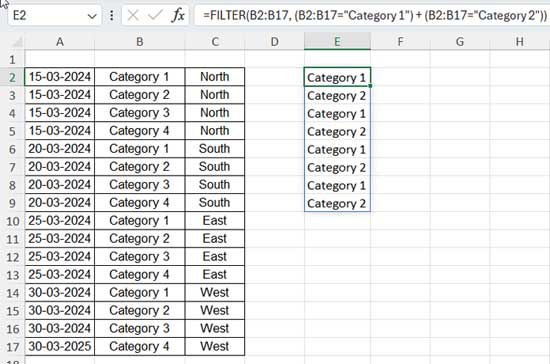

Even though we include two criteria, for the FILTER function, it’s interpreted as only one condition, which is an array containing TRUE (1) or FALSE (0) values.

AND Criteria (Matching All the Criteria):

Example 1:

To extract the rows in B2:C17 that match “Category 1” in the “North” region, we can use the following formula in both Excel and Google Sheets:

=FILTER(B2:C17, (B2:B17="Category 1") * (C2:C17="North"))

Although there are two criteria, for the FILTER function, it interprets them as a single array containing TRUE or FALSE values.

While this formula works in Google Sheets, you can also use two conditions separately, like this:

=FILTER(B2:C17, B2:B17="Category 1", C2:C17="North")

However, Excel doesn’t support this approach as it has only one argument for the criterion, i.e., include.

Example 2:

The following formula filters the array A2:A17 where the dates in column A are between today’s date and today’s date plus 10:

=FILTER(A2:A17, (A2:A17 > TODAY()) * (A2:A17 < TODAY() + 10))

This formula will work in both Excel and Google Sheets. However, in Google Sheets, you can also use the following formula, which won’t work in Excel:

=FILTER(A2:C17, A2:A17 > TODAY(), A2:A17 < TODAY() + 10)

Comparing AND and OR Usage in the FILTER Functions: Excel vs. Google Sheets

To extract rows in B2:C17 based on “Category 1” from “North” or “South” regions, you can use the following formula in both applications:

=FILTER(B2:C17, (B2:B17="Category 1") * ((C2:C17="North") + (C2:C17="South")))

However, in Google Sheets, if you prefer, you can separate the AND criterion part as follows:

=FILTER(B2:C17, B2:B17="Category 1", ((C2:C17="North") + (C2:C17="South")))

Conclusion

In short, if you omit the last argument in the Excel FILTER function, i.e., if_empty, it will work flawlessly in Google Sheets.

Additionally, it’s worth noting that there’s a minor difference when the range to filter contains dates: the FILTER function in Excel returns date values, while Google Sheets returns the dates themselves. However, if you use IFNA with FILTER, it will also return date values.

That concludes the comparison of the FILTER function in Excel and Google Sheets.