The core purpose of the SUMPRODUCT function remains consistent across both Excel and Google Sheets. It multiplies corresponding items from two or more arrays and then sums those products.
However, the usage of the SUMPRODUCT function differs slightly between Excel and Google Sheets, particularly when applying conditions.
In addition, the array formula capability of SUMPRODUCT in Excel is exemplary, especially in Excel legacy formulas. It can be utilized to iterate over each value in an array in certain calculations. I’ll provide an example in the later part of this tutorial.
Google Sheets SUMPRODUCT doesn’t have this functionality. However, it’s no longer necessary, after LAMBDAS.
Boolean Value Handling: The Core Reason for SUMPRODUCT Usage Differences
Let’s first understand how SUMPRODUCT handles Boolean TRUE and FALSE values in multiplication. This will help us grasp the usage differences.
Suppose we have the following values in cells A1:B3 in both Excel and Google Sheets:
| TRUE | 10 |
| FALSE | 15 |
| TRUE | 20 |
The syntax of the SUMPRODUCT function is SUMPRODUCT(array1, [array2, …]).
The following formula in Google Sheets will return 30, whereas in Excel, it will return 0:
=SUMPRODUCT(A1:A3, B1:B3)In Google Sheets, SUMPRODUCT reads or assigns 1 to TRUE and 0 to FALSE. So, the total of 1*10 + 0*15 + 1*20 will be 30.
In Excel, you need to coerce Boolean values into their numeric equivalents using one of the techniques below:
- double dash:
=SUMPRODUCT(--A1:A3, --B1:B3) - multiplying:
=SUMPRODUCT(A1:A3 * 1, B1:B3 * 1)or=SUMPRODUCT(A1:A3 * B1:B3)
When applying conditions to a range, for example, A1:A100=”Apple”, the formula returns TRUE or FALSE. This causes issues in Excel SUMPRODUCT, not in Google Sheets. The above methods address this in Excel. Here is a real-life example.
Example
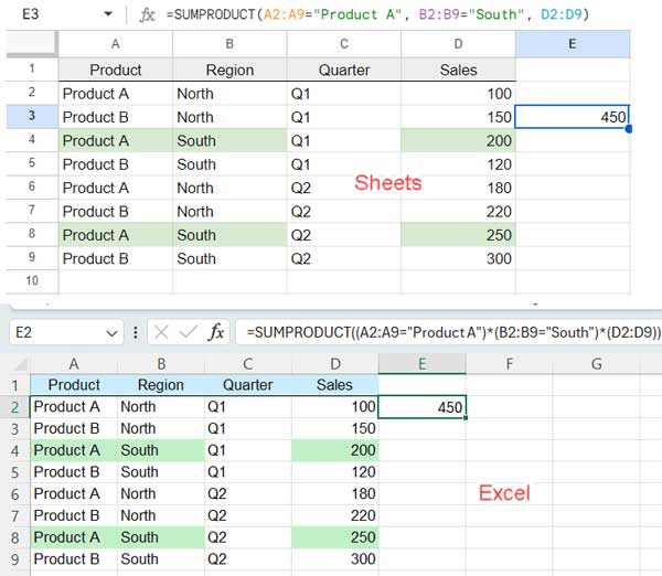
Columns A to D contain Product, Region, Quarter, and Sales. The data range is A2:D9.
How to return the total sales of “Product A” in the “South” region?
In Google Sheets, you can use the following formula:
=SUMPRODUCT(A2:A9="Product A", B2:B9="South", D2:D9)In Excel, you have a few options:
=SUMPRODUCT((A2:A9="Product A")*1, (B2:B9="South")*1, D2:D9)
=SUMPRODUCT((A2:A9="Product A")*(B2:B9="South"), D2:D9)
=SUMPRODUCT((A2:A9="Product A")*(B2:B9="South")*(D2:D9))
All these formulas will work in Google Sheets as well.
That is the difference between SUMPRODUCT in Excel and Google Sheets.
The Role of SUMPRODUCT in Legacy Array Formulas in Excel
The above formulas return the total sales of “Product A” in the “South” region. How do we exclude rows in the range that are hidden in this calculation?
Currently, there are no hidden rows. However, if I hide a row, I want the formulas to return the total of visible rows.
In older versions of Excel, you can use the following formula:
=SUMPRODUCT((A2:A9="Product A")*(B2:B9="South")*(SUBTOTAL(103, OFFSET(A2, ROW(A2:A9)-ROW(A2), 0)))*(D2:D9))The formula is the same, but there is a new array included which is SUBTOTAL(103, OFFSET(A2, ROW(A2:A9)-ROW(A2), 0)).
What does this formula do?
It copies =SUBTOTAL(103, A2) to each row. It returns 1 in each visible row and 0 in each hidden row wherever a value is present in A2:A9. The function number 103 in SUBTOTAL is equal to COUNTA but skips hidden values.
This formula will work in Excel for Microsoft 365 as well but not in Google Sheets. In Google Sheets, you can replace the above-highlighted part with the following lambda function:
MAP(A2:A9, LAMBDA(r, SUBTOTAL(103, r)))This will also work in Excel for Microsoft 365.
Conclusion
Understanding the nuances of how Excel and Google Sheets handle SUMPRODUCT, especially with Boolean values and array formulas, ensures your spreadsheets function smoothly on both platforms, maximizing the utility of this powerful function.
Resources
- Subtotal Function With Conditions in Excel and Google Sheets
- Array Formula: How It Differs in Google Sheets and Excel
- Grouping and Subtotal in Google Sheets and Excel
- Comparing the FILTER Function in Excel and Google Sheets
- Google Sheets Vs Excel: BYROW – The Key Difference
- BYCOL Differences: Sheets vs. Excel


