The SUBTOTAL function is useful for aggregating values in visible rows but doesn’t natively support conditions. This tutorial covers how to use SUBTOTAL with conditions in Excel and Google Sheets, with and without helper columns.
Excel has a slight edge here, as it doesn’t require a LAMBDA function to avoid using helper columns, whereas Google Sheets relies on LAMBDA for a similar outcome.
However, this doesn’t mean Excel is universally better—Google Sheets’ LAMBDA approach works in scenarios that Excel’s implementation may not cover.
It’s important to note that conditional functions like COUNTIF, SUMIF, MINIFS, MAXIFS, and AVERAGEIFS in both Google Sheets and Excel don’t automatically exclude filtered or hidden rows.
To aggregate only visible rows conditionally, we’ll use SUBTOTAL as an additional criterion. Excel uses an OFFSET-based SUBTOTAL, while Google Sheets relies on a LAMBDA-based SUBTOTAL approach.
Introduction to the SUBTOTAL Function in Excel and Google Sheets
The SUBTOTAL function is a flexible tool for aggregating data across a range using specific functions. The function’s versatility comes from its ability to apply various operations by using function numbers, which allow it to perform calculations only on visible rows or on all data.
| Aggregate Function | Filtered Only (#) | Hidden & Filtered (#) |
| AVERAGE | 1 | 101 |
| COUNT | 2 | 102 |
| COUNTA | 3 | 103 |
| MAX | 4 | 104 |
| MIN | 5 | 105 |
| PRODUCT | 6 | 106 |
| STDEV | 7 | 107 |
| STDEVP | 8 | 108 |
| SUM | 9 | 109 |
| VAR | 10 | 110 |
| VARP | 11 | 111 |
In the following examples, we will use function numbers 3 or 103 to create a physical or virtual helper column for conditional aggregation.
We’ll explore examples of using SUBTOTAL for conditionally counting, summing, finding minimums, maximums, and calculating averages on visible rows.
Using SUBTOTAL with Conditions in Excel and Google Sheets: Helper Column Approach
While the SUBTOTAL function doesn’t natively support conditions (like a hypothetical SUBTOTALIF might), a helper column can serve as an effective workaround. Here’s how to set it up:
Our sample data consists of product names in column A, area in column B, and amounts in column C, covering the range A1:C11.
In this example, we’ll use column D as the helper column. Enter one of the following formulas in cell D2, then drag it down to D11:
=SUBTOTAL(103, A2)// Use this to omit both hidden and filtered rows=SUBTOTAL(3, A2)// Use this to omit only filtered rows
You do not need to stick to A2; you can use B2 or C2 as the first-row reference within the range. However, it is recommended to choose a reference from a column without blank cells for more accurate results.
When you hide a row, the value in that row in column D becomes 0. Thus, 0 indicates a hidden row and 1 indicates a visible row. We will use this as the criteria for our calculations.
Conditional Formulas Using SUBTOTAL with a Helper Column
Here’s how to use aggregation functions with visible rows in Excel and Google Sheets, based on the helper column:
Average Visible Rows
=AVERAGEIFS(C2:C11, D2:D11, 1, A2:A11, "Apple")Note: In the above formula and the following formulas, A2:A11 and D2:D11 are the criteria ranges, and “Apple” and 1 are the respective criteria.
Count Visible Rows
=COUNTIFS(D2:D11, 1, A2:A11, "Apple")Minimum of Visible Rows
=MINIFS(C2:C11, D2:D11, 1, A2:A11, "Apple")Maximum of Visible Rows
=MAXIFS(C2:C11, D2:D11, 1, A2:A11, "Apple")Sum of Visible Rows
=SUMIFS(C2:C11, D2:D11, 1, A2:A11, "Apple")These formulas aggregate only visible rows and are enhanced by applying conditions to the helper column.
Using SUBTOTAL with Conditions in Excel and Google Sheets: Without a Helper Column Approach
Excel:
In Excel, it’s possible to create a dynamic helper column without explicitly entering one.
=SUBTOTAL(103, OFFSET(A2, ROW(A2:A11) - ROW(A2), 0))This approach mirrors entering the following formula D2 and dragging it down:
=SUBTOTAL(103, OFFSET(A2, 0, 0))To perform aggregation directly in Excel without a helper column, use the following formulas:
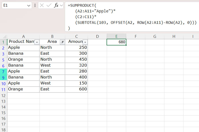
Sum of Visible Rows with Criteria
=SUMPRODUCT(
   (A2:A11="Apple")*
   (C2:C11)*
   (SUBTOTAL(103, OFFSET(A2, ROW(A2:A11)-ROW(A2), 0)))
)
Count Visible Rows with Criteria
=SUMPRODUCT(
   (A2:A11="Apple")*
   (SUBTOTAL(103, OFFSET(A2, ROW(A2:A11)-ROW(A2), 0)))
)
Maximum of Visible Rows with Criteria
For versions of Excel that do not support dynamic array formulas, enter this as an array formula by pressing Ctrl + Shift + Enter:
=MAX(
   IF(
      A2:A11="Apple",
     (C2:C11)*(SUBTOTAL(103, OFFSET(A2, ROW(A2:A11) - ROW(A2), 0))),
      ""
   )
)
Minimum of Visible Rows with Criteria
For minimum calculations, it’s best to use a helper column formula; otherwise, it may return 0 as the minimum when rows are hidden.
Average of Visible Rows with Criteria
For the average, you can divide the sum by the count using the respective formulas above, or you can use a helper column for simplicity.
Google Sheets:
In Excel, we used an OFFSET-based formula to apply SUBTOTAL without helper columns. However, this approach doesn’t work in Google Sheets.
Instead, you can use the following formula to replace the helper range D2:D11 in all formulas under the “Conditional Formulas Using SUBTOTAL with Helper Column” section:
=MAP(A2:A11, LAMBDA(row, SUBTOTAL(103, row)))For example, we can replace the helper column formula in:
=AVERAGEIFS(C2:C11, D2:D11, 1, A2:A11, "Apple")with:
=AVERAGEIFS(C2:C11, MAP(A2:A11, LAMBDA(row, SUBTOTAL(103, row))), 1, A2:A11, "Apple")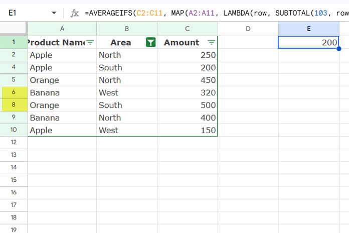
This provides a method for using the SUBTOTAL function with conditions in both Excel and Google Sheets. Let me know if you have questions about any of these functions!


Hi,
Will count text values work in this logic?
Hi, Jay,
We can try with a sample. Feel free to share a demo sheet below as I won’t publish it.
OMG. Thank you for this. I too was searching for a solution.
Hi, Tia Zhan,
Thank you for leaving your feedback.
Not sure if you’re still monitoring replies, but I wanted to thank you for this nifty little trick.
This solved a problem I was trying to solve with very complicated nested IFs. And even though I was convinced that there was a simpler way, I didn’t see how.
The simple addition of the helper column saved me a lot of time.
Thank you for sharing this.