The LAMBDA function in Google Sheets lets you define and use a custom function on its own, without needing to pair it with helper functions like MAP or REDUCE. While it’s commonly used with helper functions—such as MAP, REDUCE, and BYROW—this post focuses solely on its standalone use. You’ll also learn how to assign a name using LET so you can reuse your LAMBDA function.
Although this post is focused on standalone use, I’ve included links to related tutorials—covering MAP, REDUCE, BYROW, and others—at the end of the page in case you’d like to explore them later.
If you’re already familiar with the LAMBDA function in Excel, you’re off to a great start. As far as I know, its usage is identical in both Excel and Google Sheets.
In Excel, we use the LAMBDA function both with helper functions and within the Name Manager to create reusable custom functions.
In Google Sheets, LAMBDA is also used with helper functions, but there’s no Name Manager. Instead, Google Sheets offers Named Functions (found under the Data menu), which don’t necessarily require LAMBDA.
In this post, we’ll focus on using the LAMBDA function in Google Sheets as a standalone tool. Once you’re comfortable with that, you’ll find it easier to understand how it works with its helper functions later on.
LAMBDA Function Syntax and Arguments (Standalone Use)
Syntax:
=LAMBDA([name, ...], formula_expression)(function_call, ...)Arguments:
- name – An optional identifier (or multiple, comma-separated identifiers) to pass values to the formula.
- The name must be valid — it can’t be a cell reference like
A1orB1. - Special characters are not allowed (except dots and underscores).
- Names can’t start with numbers.
- The name must be valid — it can’t be a cell reference like
- formula_expression – The actual formula you want to calculate or execute. This is a required argument.
- function_call – The values or references passed to the function. If no
nameis defined, you simply use().
Note: If you check the official documentation for the LAMBDA function in Google Sheets, the syntax might look slightly different. I’ve rewritten it here for clarity.
LAMBDA Function Examples in Google Sheets
Here are a few examples to help you understand how the LAMBDA function works. At first, you might wonder why you’d even need this function — but its true potential becomes clear when paired with helper functions. We’ll cover those in future tutorials.
Examples Without the Optional Name Argument
As mentioned earlier, the name argument is optional. If you’re not passing any value into the formula, you can skip it.
Example 1 (Non-Array Formula)
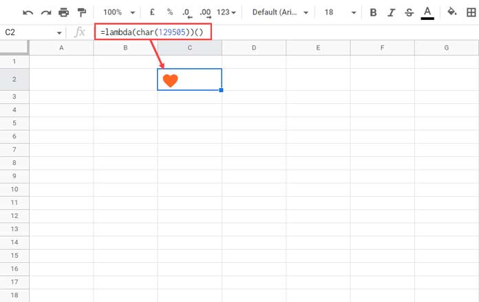
This regular formula returns a heart character:
=CHAR(129505)🧡 (Output)
Since there are no references or inputs, we can create a LAMBDA version like this:
=LAMBDA(CHAR(129505))()CHAR(129505)is the formula_expression()is the function_call
Example 2 (Array Formula)
If you insert the following formula in cell B1, and if the range B1:B10 is empty, it will return the numbers 1 to 10 in that column:
=ARRAYFORMULA(ROW(A1:A10))This formula uses ROW(A1:A10) to generate the numbers 1 to 10, and ARRAYFORMULA ensures they spill vertically into B1:B10.
Converted to a LAMBDA function:
=LAMBDA(ARRAYFORMULA(ROW(A1:A10)))()Examples Using All LAMBDA Arguments
Now let’s pass values into the function using the name argument.
Example 3 (Non-Array Formula)
Enter 5 in cell A1. Then enter this formula elsewhere:
=REPT(CHAR(129505), A1)🧡🧡🧡🧡🧡 (Output)
Now, the LAMBDA version:
=LAMBDA(n, REPT(CHAR(129505), n))(A1)nis the name (input)REPT(CHAR(129505), n)is the formula_expressionA1is the function_call
Example 4 (Array Formula)
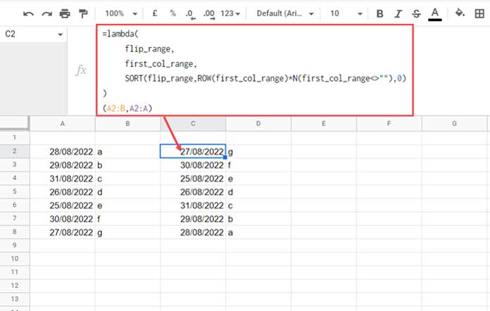
Let’s flip data in a range using SORT.
Say your data is in A2:B, and you want to flip it.
Place the following in cell C2 (leave C2:D empty):
=SORT(A2:B, ROW(A2:A) * N(A2:A <> ""), 0)LAMBDA version:
=LAMBDA(
   flip_range,
   first_col_range,
   SORT(flip_range, ROW(first_col_range) * N(first_col_range <> ""), 0)
)(A2:B, A2:A)flip_rangeandfirst_col_rangeare the names (inputs)SORT(...)is the formula_expressionA2:B, A2:Aare the actual inputs in the function_call
Reuse a LAMBDA Function Using LET
You can reuse a LAMBDA function by naming it with LET.

Original LAMBDA Formula:
=LAMBDA(
   name,
   score,
   FILTER(name, score >= 90)
)(B2:B, C2:C)
This filters student names from B2:B where their scores in C2:C are 90 or above.
Step 1: Name the LAMBDA with LET
=LET(ftr,
   LAMBDA(
      name,
      score,
      FILTER(name, score >= 90)
   ), ftr(B2:B, C2:C)
)
Now ftr is your reusable custom function.
Step 2: Reuse It with New Ranges
=LET(
   ftr,
   LAMBDA(
      name,
      score,
      FILTER(name, score >= 90)
   ), VSTACK(ftr(B2:B, C2:C), ftr(E2:E, F2:F))
)
Here, we use ftr twice — once for the first range, and again for another set of data — and stack the results vertically using VSTACK.
Common Errors
| Error | What It Means |
|---|---|
#N/A | The formula is missing the function_call (actual inputs). |
#NAME? | Invalid identifier or incorrect function name used in the formula. |
#REF! | Circular dependency or referencing issue. |
That’s all about how to use the LAMBDA function in Google Sheets in standalone mode.
Thanks for reading. Enjoy experimenting!
Related Resources
- How to Use the REDUCE Function in Google Sheets
- How to Use the SCAN Function in Google Sheets
- How to Use the MAP Function in Google Sheets
- How to Use the BYCOL Function in Google Sheets
- How to Use the BYROW Function in Google Sheets
- How to Use the MAKEARRAY Function in Google Sheets
- Excel LAMBDA: Creating Named and Unnamed Custom Functions


