This post is about the MAKEARRAY Lambda function in Google Sheets. It requires a LAMBDA or a Named Function as input.
When I went through the list of the Lambda helper functions BYROW, BYCOL, SCAN, REDUCE, MAP, and MAKEARRAY, I thought the MAKEARRAY was the least helpful LHF. But it does also have the wow factor.
For example, we will get “range must be a single row or a single column” when we try to apply a MATCH formula to an entire table.
=match("Name",A1:D4,0)Here I could use the MAKEARRAY function in combination with a named function to make the MATCH formula to use every row in a table.
We will see that example at the end part of this Google Sheets tutorial.
I’ve also included an example of expanding a conditional DMAX to every row using this new function.
=dmax($A$1:$C,3,{"Rank";B2})Dragging this formula (cell spill handle) down will change the cell reference B2 to B3, B3 to B4, and so on. We can make it auto-spill.
All the LHFs are equally important. They have their roles in making our spreadsheet tasks simpler.
MAKEARRAY Purpose: Returns a calculated array of specified dimensions (specified row and column size) by applying a LAMBDA.
MAKEARRAY Function Syntax and Arguments
Syntax:
MAKEARRAY(rows, columns, LAMBDA)Where;
rows – The number of rows in the output array.
columns – The number of columns in the output array.
LAMBDA – A LAMBDA that takes two names for rows and columns to create the array.
Syntax: =LAMBDA(name1, name2,formula_expression)(function_call, …)
Note:- The highlighted part is not required when using it in the MAKEARRAY function.
name1 – The row index of the array.
name2 – The column index of the array.
Understand the MAKEARRAY Function in Google Sheets
We use the MAKEARRAY function to return calculated arrays, so it’s simple to use.
But you must first understand what it returns in columns and rows without calculation.
Assume the row index is three and the column index is two.
The array without calculation from the perspective of row index:
| 1 | 1 |
| 2 | 2 |
| 3 | 3 |
And from the perspective of column index:
| 1 | 2 |
| 1 | 2 |
| 1 | 2 |
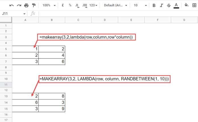
So the output of the following MAKEARRAY formula in Google Sheets will be as per the table below.
=makearray(3,2,lambda(row,column,row*column))| 1*1=1 | 1*2=2 |
| 2*1=2 | 2*2=4 |
| 3*1=3 | 3*2=6 |
And if you use =MAKEARRAY(3,2, LAMBDA(row, column, RANDBETWEEN(1, 10))), it will return a 3 x 2 matrix filled with random numbers from 1 to 10.
How to Use MAKEARRAY With Named Functions in Google Sheets
In the following examples, we will create two Named Functions to expand the result of MATCH and DMAX.
I hope that will make you understand the potential of the MAKEARRAY function in Google Sheets.
1. Match a Value in Every Row
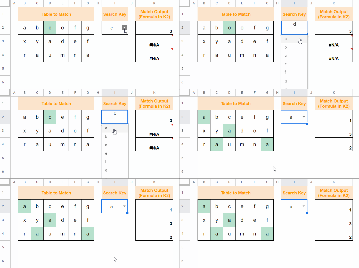
How to match the search key in I2 in B2:G2, B3:G3, and B4:G4?
Usually, we will use the following formula in K2 and drag it down since the MATCH function won’t accept more than one row or column as its range.
=match($I$2,B2:G2,0)But here in the above example, I created a Named Function called TEST and used that within the MAKEARRAY Function.
The MAKEARRAY formula in K2 that expands the MATCH result to K2:K4 is as follows.
=makearray(3,1,TEST)And what about the TEST function in use?
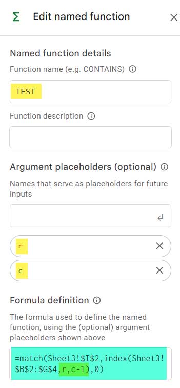
The TEST function takes two arguments – r (row) and c (column).
When you use the TEST function stand-alone, you must use three formulas in K2:K4.
They are =TEST(1,1), =TEST(2,1), and, =TEST(3,1).
The MAKEARRAY feeds the arguments within the TEST function at one go as it returns a 3×1 array.
2. Conditional DMAX in Every Row
Here is one more MAKEARRAY function example in Google Sheets to make you understand how useful it is to spill (expand) formula results.
This time we have a database function in use.
Problem:
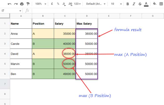
The first three columns in the above table contain employee information such as name, position, and salary.
In the last column, I want to assign the maximum salary drawn in each “position” to each employee.
For example, the maximum salary drawn for position “A” is 38000.
So I want to assign this salary amount to “Anna,” and “David” as they belong to that position.
Solution:
We usually use the following DMAX in cell D2 and copy-paste it down.
=dmax($A$1:$C$6,3,{"Position";B2})Let’s see how to make it an array formula using the MAKEARRAY function in Google Sheets.
Let’s first create a Named Function called DTEST, which is as follows.
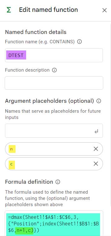
Then we can use the following formula in cell D2 which will spill down.
=MAKEARRAY(5,1,DTEST)That’s all. Thanks for the stay. Enjoy!


Oh, awesome! I didn’t realize those other two were so easy! That is a lot simpler structure than the Makearray version. I’ll have to update some of my recent projects to test out those two. Thanks for sharing!
Thanks for the quick and detailed explainer. I’ve taken what you’ve shown and tested that the pattern also works to turn any of the SUM, SUMIFS and other aggregation functions into array formulas.
The structure is definitely cumbersome and likely too complex for most, but at least it makes it possible. So that is a major improvement.
For a real game-changer though, turn this into a Named Range, and you can now run GOOGLEFINANCE calls with a single array formula!
=MAKEARRAY(ROWS(range),1, LAMBDA(r,c, GOOGLEFINANCE( INDEX(range,r,c), "price") ))Hi, McKay Savage,
Thanks for your feedback.
We can easily make most of the non-array formulas into array formulas by using the BYROW or MAP functions.
Instead of the above MAKEARRAY formula, we can use the following BYROW formula.
=byrow(B2:B10,lambda(ticker, ifna(GOOGLEFINANCE(ticker,"price"))))Using MAP:
=map(B2:B10,lambda(ticker, ifna(GOOGLEFINANCE(ticker,"price"))))Where; B2:B10 is that range that contains the ticker symbols or the ‘range’ as per your formula.