The REDUCE function in Google Sheets is easy to understand if you know the SCAN function. Do you know why?
Both are LAMBDA helper functions (LHFs) and apply a LAMBDA to each value in the array.
The former reduces an array to an accumulated value and returns the total value in the accumulator.
The latter returns an array that has each intermediate value in the accumulator.
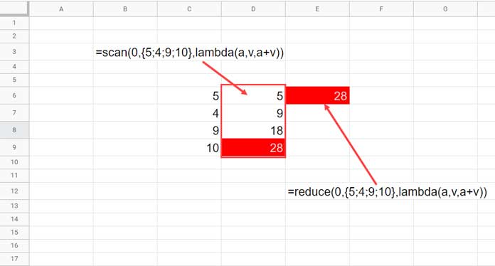
For example, the output of the following SCAN formula will be the running total, i.e., {5;9;18;28}.
=scan(0,{5;4;9;10},lambda(a,v,a+v))If you use the following REDUCE formula, you will get 28, the final cell value of the above formula output, i.e., the total value in the accumulator.
=reduce(0,{5;4;9;10},lambda(a,v,a+v))Understanding the above difference may help you choose the correct LHF to solve your problem in Google Sheets.
REDUCE Function Syntax and Arguments in Google Sheets
Reduce Syntax:
REDUCE(initial_value, array_or_range, LAMBDA)Where;
initial_value – To set the initial/starting value of the accumulator.
array_or_range – An array or range to be reduced.
LAMBDA – A LAMBDA that’s called to reduce the array_or_range. It takes two name arguments.
LAMBDA Syntax: =LAMBDA([name, ...],formula_expression)(function_call, ...)
Note: We are only required to use the function_call argument in standalone LAMBDA use. Please check my Google Sheets function guide to learn this function.
We can read the syntax for the REDUCE function as LAMBDA(name1, name2, formula_expression).
Where name1 is the accumulator and name2 is the calculation applied to each element in the array_or_range.
To better understand the syntax of the REDUCE function in Google Sheets, please try the examples below.
How to Use the REDUCE Function in Google Sheets
In the beginning, we have seen two examples of using the SCAN and REDUCE Lambda Helper Functions (LHFs) in Google Sheets.
Let’s see them in a Google Sheets spreadsheet and compare.

Both functions have the same arguments: initial_value, array_or_range, and LAMBDA, and here are them in the formula.
initial_value – 0
array_or_range – {5;4;9;10} or you can use B2:B also.
LAMBDA (LAMBDA(name1, name2, formula_expression)
name1 – a (accumulator)
name2 – v (the calculation applied to each element in the array)
The SCAN in cell D6 returns the accumulator value against each element in the array, whereas the REDUCE in E6 returns the final value in the accumulator.
So we can use them in different scenarios.
For example, we can use the SCAN LHF for (conditional) running totals and REDUCE LHF for (conditional) count or sum.
Examples (LHF for Conditional Count and Sum)
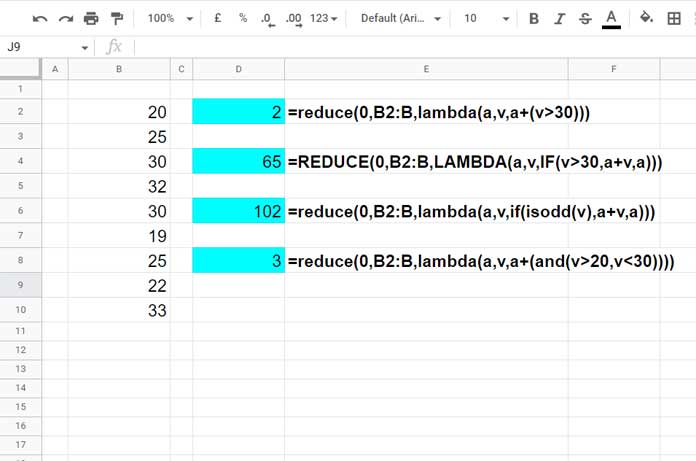
Below you can find four REDUCE LAMBDA Helper function (LHF) examples. I’ll explain them one by one.
In all the examples, the initial value of the accumulator is 0 (zero).
If we set it as 100 as an example, the outputs in the Cyan highlighted cells will be 102, 165, 202, and 103, respectively.

1. REDUCE Function for Conditional Sum
The D4 and D6 formulas are examples of using the REDUCE function for conditional sum.
The following D4 formula sums B2:B (array_or_range) if the values in this array are >30.
=REDUCE(0,B2:B,LAMBDA(a,v,IF(v>30,a+v,a)))It’s equal to using a SUMIF as below.
=sumif(B2:B,">30")The formula applies v>30 to each element in the array. The IF function does that logical test.
If it evaluates to TRUE, it performs a+v (adds the value to the accumulator) else retains a, the accumulator value.
It does this in the whole column and returns the final value called reduced array result.
The following D6 formula adds odd values and returns the total.
=reduce(0,B2:B,lambda(a,v,if(isodd(v),a+v,a)))SUMIF Alternative: =ArrayFormula(sumif(isodd(B2:B),TRUE,B2:B))
The above are examples of using the REDUCE function for conditional sums in Google Sheets.
2. Reduce Function for Conditional Count
The other two formulas in D2 and D8 act as conditional counts.
Assume the values in B2:B are the age of participants in a competition.
The D2 formula returns the counts of participants above the age of 30.
=reduce(0,B2:B,lambda(a,v,a+(v>30)))It is equal to using the following COUNTIF in Google Sheets.
=countif(B2:B,">30")The second REDUCE formula in cell D8 acts as a COUNTIFS formula which returns the number of participants in the age group 20 to 30.
=reduce(0,B2:B,lambda(a,v,a+(and(v>20,v<30))))Here is the COUNTIFS alternative.
=countifs(B2:B,">20",B2:B,"<30")Other Use Cases
Going through the examples above, you may fall under the false impression that the REDUCE function doesn’t require much attention.
You are wrong if that’s the case!
We can use this Google Sheets LAMBDA helper function not only for count or sum based on conditions. It has other uses.
For example, the below REDUCE function-based formula can return the last value in numeric column B.
=reduce(0,B:B,lambda(a,v,(if(v="",v+a,v))))To return the last value in row # 2 (numeric), just replace B:B with 2:2.
If you have mixed type values, replace the initial_value , i.e., 0, with "" and v+a with v&a.
The following REDUCE formula will total column B if column A values are “apple.”
=reduce(0,A:A,lambda(a,v,if(v="apple",offset(v,0,1)+a,a)))You can use such formulas to create shorter named functions also.


