Google Sheets SUMIF Function: Complete Guide with Examples

The SUMIF function in Google Sheets is one of the most widely used spreadsheet functions for conditional summation. It is easy to learn, yet powerful enough for many advanced calculations.

You can use SUMIF to total sales for a product, sum values above a number, calculate totals for a month, summarize stock movement, and much more.

This tutorial is a complete guide to using the SUMIF function in Google Sheets. It starts with the basics and then links to advanced tutorials that solve real-world SUMIF challenges.

Table of Contents

What Is the SUMIF Function in Google Sheets?

The main purpose of the SUMIF function is conditional summation.

It adds values in a range based on a condition in the same range or another range.

For example, you can:

Sum only TV sales
Total quantities sold in December
Add numbers greater than 100
Sum values beginning with specific text
Create quick summary reports

Because of its simplicity, SUMIF remains one of the most practical formulas in Google Sheets.

SUMIF Syntax and Arguments

SUMIF(range, criterion, [sum_range])

Arguments

range

The cells tested against the condition.

This can be:

A normal range like A2:A100
An expression returned by another formula (such as IMPORTRANGE)

criterion

The condition applied to the range.

Examples:

"TV"
100
">=50"
DATE(2026, 4, 1)

sum_range (optional)

The cells to add.

Use this when the values to total are in a different column. The sum_range must point to actual cells on the sheet, not to the result of another formula.

Basic SUMIF Examples

Suppose the data in A1:C6 is:

Product Name	Date	Qty Sold
TV	01/10/2017	10
TV	15/11/2017	3
Projector	15/11/2017	2
Projector	15/12/2017	3
TV	15/12/2017	7

Qty Sold > 5

=SUMIF(C2:C6, ">5")

Here, we have not used the sum_range argument because the criteria range and sum range are the same. In such cases, SUMIF adds the matching values directly from the range itself.

Total TV Units Sold

=SUMIF(A2:A6, "TV", C2:C6)

Total Projector Units Sold

=SUMIF(A2:A6, "Projector", C2:C6)

Use a Cell Reference for Criteria

If E2 contains TV:

=SUMIF(A2:A6, E2, C2:C6)

This is usually better than hardcoding text inside formulas.

Important Notes

SUMIF is not case-sensitive.
Text criteria need double quotes.
Numbers do not need double quotes.
Dates are best entered using the DATE() function with the syntax DATE(year, month, day).

SUMIF with Dates

To total quantities sold on 15 November 2017:

=SUMIF(B2:B6, DATE(2017, 11, 15), C2:C6)

SUMIF Array Formula

You can return totals for multiple criteria at once.

=ARRAYFORMULA(SUMIF(A2:A6, {"TV";"Projector"}, C2:C6))

Using Cell References:

=ARRAYFORMULA(SUMIF(A2:A6, E2:E3, C2:C6))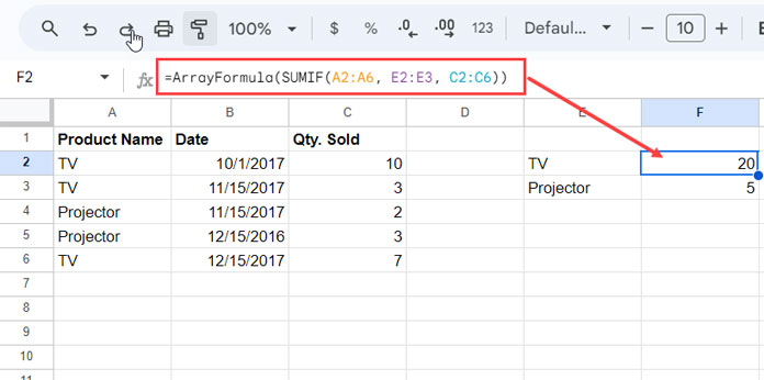

ARRAYFORMULA SUMIF in Google Sheets returning separate totals for criteria listed in cells E2:E3

These formulas return two separate values, one for each criterion.

If you want the combined total instead, replace the ARRAYFORMULA wrapper with SUMPRODUCT:

=SUMPRODUCT(SUMIF(A2:A6, E2:E3, C2:C6))

Comparison Operators and Wildcards

Sum Values on or After a Date

=SUMIF(B2:B6, ">="&DATE(2017, 12, 1), C2:C6)

Sum Quantities Greater Than 2

=SUMIF(C2:C6, ">2")

Wildcard Example

Sum products beginning with “pr”:

=SUMIF(A2:A6, "pr*", C2:C6)

Wildcards:

* any number of characters
? one character

Real-Life Example of SUMIF

SUMIF is excellent for creating summary sheets.

Suppose cable transactions are recorded in Sheet1, range A3:E, with the following fields:

Item Code
Item Description
Qty. Received from Client Store in Mtr.
Issued to Employee
Balance

Sheet1 cable receipt data in Google Sheets showing item code, item name, quantity received, issued, and balance

Now you want to create a summary report in Sheet2.

Step 1: Get Unique Item Names

Enter the following formula in Sheet2!B4 to return the unique cable names:

=UNIQUE(Sheet1!B4:B)

Sheet2 cable receipt summary in Google Sheets showing item-wise totals using SUMIF formulas

Step 2: Create Stock Balance Summary

Enter the following formulas in Sheet2!C4, D4, and E4 respectively:

=ARRAYFORMULA(SUMIF(Sheet1!B4:B, B4:B, Sheet1!C4:C))

=ARRAYFORMULA(SUMIF(Sheet1!B4:B, B4:B, Sheet1!D4:D))

=ARRAYFORMULA(C4:C-D4:D)

This instantly creates a stock summary for each item.

Sample Sheet

You can copy and test this example using the sample Google Sheet below:

Sample Sheet

Advanced SUMIF Tutorials

Core Usage

Criteria & Conditions

Dates & Time

Ranges & Structure

Filters, Hidden Rows & Arrays

Multi-Sheet / External Data

Advanced Alternatives & Techniques

SUMIF with Other Google Sheets Features

Common Errors and Fixes

Mismatched Data Types

If criteria are text, ensure the matching range also contains text values.

Blank Cells in Date Range

Using a month number (such as 12) directly as the criterion on a date column may also include rows where the date cells are blank, leading to unintended totals.

Extra Spaces in Data

Imported or manually entered text may contain spaces.

Use:

Data → Data clean-up → Trim whitespace

Common Error Messages

#ERROR!

Formula parse issue. Check commas or separators.

#N/A Argument Must Be a Range

Usually happens when sum_range is not a physical range.

#REF!

Can happen when array results do not have room to expand.

SUMIF vs SUMIFS

Function	Best For
SUMIF	Applying one condition
SUMIFS	Applying multiple conditions across one or more columns

Use SUMIF when you only need a single condition, such as totaling sales for TV.

=SUMIF(A2:A10, "TV", C2:C10)

Use SUMIFS when you need multiple conditions, such as totaling TV sales in December.

=SUMIFS(C2:C10, A2:A10, "TV", B2:B10, ">="&DATE(2017, 12, 1), B2:B10, "<="&DATE(2017, 12, 31))

Conclusion

The SUMIF function in Google Sheets is one of the simplest and most effective formulas for conditional totals.

It works well for sales reports, budgets, stock summaries, dashboards, and monthly analysis.

Start with basic text and number conditions, then move to dates, month-year totals, and array formulas.

After learning SUMIF, the next useful functions to explore are SUMIFS, QUERY, and FILTER.