We can use the SUMIF function to sum multiple columns based on a criterion in Google Sheets. To achieve this, we will use a clever method in the SUMIF range part.
The SUMIF function is for summing a column based on a criterion in another column or range.
It follows the syntax SUMIF(range, criterion, [sum_range]), where range and sum_range can be 2D arrays of equal size. We will utilize this flexibility of SUMIF to sum multiple columns in Google Sheets.
Let’s start with a regular use of the SUMIF function in Google Sheets.
Sample Data:
| Description | January | February |
| Lemon | 100 | 100 |
| Lemon | 500 | 200 |
| Avocado | 400 | 100 |
| Watermelon | 500 | 200 |
The sample data consists of fruit names in A1:A5, their production quantities in January in B1:B5, and February in C1:C5.
We can use the following formula to sum the total production quantities of Lemon in January:
=SUMIF(A2:A5, "Lemon", B2:B5)Where:
range: A2:A5criterion: “Lemon”sum_range: B2:B5
To get the quantities in February, we can replace B2:B5 in the above formula with C2:C5.
How do we get the total production quantities of Lemon in both January and February using a single SUMIF formula? I mean, how can we use SUMIF with multiple sum columns?
Let’s explore that simple trick.
SUMIF with Multiple Sum Columns
Here is a clever method to include more than one sum column in the SUMIF function in Google Sheets.
Steps:
- Determine the number of columns to sum.
- Duplicate the
rangeaccording to the number of sum columns. For example, if there are 2 columns, duplicate therange2 times (Syntax –{range, range, ...}). - Use the multiple sum columns as the
sum_range.
Note: If you have several sum columns, the above method may not be practical. I’ll share a dynamic approach after this.
Example:
Based on our above ‘fruit’ data, the range is A2:A5, and the number of columns to add is two. So, we must duplicate the range A2:A5 twice. Here’s how:
{A2:A5, A2:A5}Now see the SUMIF formula:
=SUMIF({A2:A5, A2:A5}, "Lemon", B2:C5)This formula would return 900 as the output.
This method allows us to include multiple sum columns in the SUMIF function. This approach also works with Array Formulas (multiple criteria) in SUMIF. Just ensure you enter the formula as an array formula. Here is an example:
=ArrayFormula(SUMIF({A2:A5, A2:A5}, E2:E3, B2:C5))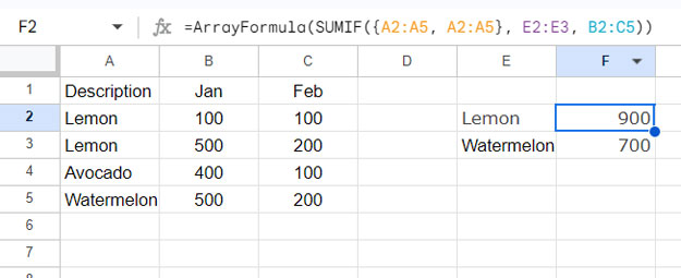
Since E2:E5 contains the fruit names ‘Lemon’ and ‘Watermelon’ (two criteria), the formula returns two values.
Have Several Sum Columns? Here’s a Cool Hack to Repeat the Range
When you have several sum columns to include in the SUMIF, the above array approach may not be practical.
For example, if you have 12 columns from January to December as sum_range and one range, you would need to use the range as {range, range, range, range, range, range, range, range, range, range, range, range}.
This can make the formula cumbersome and difficult to manage. Here is a solution to this problem:
Instead of specifying the array as above, you can use this formula:
VLOOKUP(range, range, 1, SEQUENCE(1, n, 0, 0))This VLOOKUP formula will repeat the range as many times as you want. You just replace ‘n’ with the number of times to repeat the range.
When using this formula, you should enter the SUMIF as an array formula, regardless of the number of criteria you use.
For example, we can replace our above SUMIF two columns formula with the following one:
=ArrayFormula(SUMIF(VLOOKUP(A2:A5, A2:A5, 1, SEQUENCE(1, 2, 0, 0)), E2:E3, B2:C5))Where:
range: SUMIF(VLOOKUP(A2:A5, A2:A5, 1, SEQUENCE(1, 2, 0, 0))criterion: E2:E3sum_range: B2:C5
Resources
- How to Use Dynamic Ranges in SUMIF Formula in Google Sheets
- How to SUMIF When Multiple Criteria in the Same Column in Google Sheets
- Multiple Criteria SUMIF Formula in Google Sheets (Beyond Basic SUMIF)
- How to Include Adjacent Blank Cells in SUMIF Range in Google Sheets
- Using SUMIF in a Text and Number Column in Google Sheets
- The Sum of Matrix Rows or Columns Using SUMIF in Google Sheets
- Dynamic Sum Column in SUMIF in Google Sheets


