The SUMIFS function in Google Sheets can handle multiple sum columns without requiring nested formulas. There is no need to look for workarounds to accomplish this.

We typically use SUMIFS to sum a column based on criteria in one or more columns of the same size. This is its primary function.

But what about using multiple sum columns in a SUMIFS function?

For instance, consider the annual sales of a few products for various projects.

Product names are listed in column A, project names are listed in column B, and the supplied quantity for each month is listed in the following twelve columns.

You want to know the supplied quantity of a specific product for a specific project in that year.

You can either add a total column at the end and use it in SUMIFS instead of the twelve monthly columns. This has a limitation, though. If you want to sum the quantity for the first quarter, this may not be helpful.

This is where the relevance of SUMIFS multiple sum columns comes in.

Logic

We should start with the syntax so that you can understand the logic of using the SUMIFS function with multiple sum columns.

Syntax:

SUMIFS(sum_range, criteria_range1, criterion1, [criteria_range2, …], [criterion2, …])

It’s important to note that the size of sum_range is determined by the size of criteria_range1.

If criteria_range1 is A1:A10, the sum_range must be of the same size, meaning it should cover 10 vertical cells.

So, if you want to use multiple sum columns, you should repeat the criteria column(s) as needed.

For example, if sum_range is C1:E10, you should repeat criteria_range1 (A1:A10) three times. This can be easily achieved using the CHOOSECOLS and SEQUENCE functions, which we will discuss below.

SUMIFS to Sum Multiple Sum Columns: Single Criteria Column

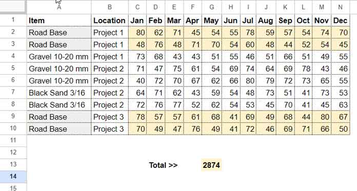
Our sample data consists of 14 columns in the range A1:N10, with A1:N1 containing the field labels. Therefore, we will use the range A2:N10 in our formulas.

Here is the structure of the sample data we have for the SUMIFS multiple sum columns test:

• A2:A10: Product Names (Road Base, Gravel 10-20 mm, and Black Sand 3/16)
• B2:B10: Location (Project 1, Project 2, and Project 3)
• C2:N10: Supplied quantity from January to December

You can click the button below to preview and copy the sample sheet.

Sample Sheet

In the above sample, I want to find the total supply of Road Base material from January to December.

How do we find it?

The following formula won’t work because the size of the criteria range and sum range are not the same. It will result in the “Array arguments to SUMIFS are of different size” #VALUE! error:

=SUMIFS(C2:N10, A2:A10, "Road Base")

Where:

• sum_range: C2:N10
• criteria_range1: A2:A10
• criterion1: “Road Base”

To make it work, we need to ensure that the dimensions of the criteria range match the sum range. The following formula accomplishes this:

ArrayFormula(CHOOSECOLS(A2:A10, SEQUENCE(12)^0))

In the SUMIFS formula, replace A2:A10 with this new formula, as follows:

=SUMIFS(C2:N10, ArrayFormula(CHOOSECOLS(A2:A10, SEQUENCE(12)^0)), "Road Base")

Where:

• sum_range: C2:N10
• criteria_range1: ArrayFormula(CHOOSECOLS(A2:A10,SEQUENCE(12)^0))
• criterion1: “Road Base”

This modified formula will correctly return the total supply of Road Base material from January to December.

This SUMIFS formula sums 12 sum columns in the range C2:N10.

Anatomy of the Formula (Criteria Range)

The CHOOSECOLS function is used to return selected columns from a range.

Examples:

CHOOSECOLS(A1:Z, 3) // returns the range C1:C
CHOOSECOLS(A1:Z, SEQUENCE(3)) // returns the range A1:C
CHOOSECOLS(A1:Z, {1, 2, 3}) // returns the range A1:C

In our SUMIFS formula, we have only one column, which is the range A2:A10, within the CHOOSECOLS. The SEQUENCE function returns the number 1, twelve times.

So, the CHOOSECOLS function returns the range A2:A10 twelve times. This way, we can match the dimension of the sum range and criteria range in the SUMIFS formula.

Here is how to use a SUMIFS formula with multiple sum columns and multiple criteria columns, specifically with a sum_range, criteria_range1, and criteria_range2.

SUMIFS to Sum Multiple Sum Columns: Multiple Criteria Columns

This time, I need to find the total sales quantity of Road Base for only Project 3.

Since there are two criteria columns, we need to handle this similarly to the above example. In addition to repeating the criteria_range1, we also need to repeat the criteria_range2 twelve times.

Here’s the formula to accomplish this:

=SUMIFS(C2:N10, ArrayFormula(CHOOSECOLS(A2:A10,SEQUENCE(12)^0)), "Road Base", ArrayFormula(CHOOSECOLS(B2:B10, SEQUENCE(12)^0)), "Project 3")

Where:

• sum_range: C2:N10
• criteria_range1: ArrayFormula(CHOOSECOLS(A2:A10,SEQUENCE(12)^0))
• criterion1: “Road Base”
• criteria_range2: ArrayFormula(CHOOSECOLS(B2:B10,SEQUENCE(12)^0))
• criterion2: “Project 3”

Note: We only need one ArrayFormula in this case, so we can shorten it as follows:

=ArrayFormula(SUMIFS(C2:N10, CHOOSECOLS(A2:A10,SEQUENCE(12)^0), "Road Base", CHOOSECOLS(B2:B10, SEQUENCE(12)^0), "Project 3"))

SUMIFS Multiple SUM Columns and REGEXMATCH

The SUMIFS function is designed to handle AND criteria.

In simple terms, you can use it to sum a sum_range where criteria_range1 equals criterion1, and criteria_range2 equals criterion2, and so forth.

To use OR criteria, some users prefer nesting SUMIFS. However, I prefer using REGEXMATCH within SUMIFS.

For example, you can use it to sum a sum_range where criteria_range1 matches criterion1. a or criterion1. b, and criteria_range2 equals criterion2, and so forth.

We have already explained the SUMIFS REGEXMATCH combination. Here’s an example before we dive into how to use SUMIFS and REGEXMATCH to sum multiple columns:

=ArrayFormula(SUMIFS(C2:C10, A2:A10, "Road Base", REGEXMATCH(B2:B10, "Project 1|Project 3"), TRUE))

Where:

• sum_range: C2:C10
• criteria_range1: A2:A10
• criterion1: “Road Base”
• criteria_range2: B2:B10
• criterion2: “Project 1” or “Project 3”

This formula returns the total supply of ‘Road Base’ for January in Project 1 and Project 3.

Note: When using REGEXMATCH with SUMIFS, make sure to use the ArrayFormula function.

Now, let’s see how to use SUMIFS with multiple sum columns in Google Sheets.

Using the same formula but for January to December, make the following changes:

• Replace A2:A10 with ArrayFormula(CHOOSECOLS(A2:A10, SEQUENCE(12)^0))
• Replace B2:B10 with ArrayFormula(CHOOSECOLS(A2:A10, SEQUENCE(12)^0))
• Finally, replace C2:C10 with C2:N10.

Here is the SUMIFS formula for multiple sum columns:

=ArrayFormula(SUMIFS(C2:N10, CHOOSECOLS(A2:A10, SEQUENCE(12)^0), "Road Base", REGEXMATCH(CHOOSECOLS(B2:B10, SEQUENCE(12)^0), "Project 1|Project 3"), TRUE))

Where:

• sum_range: C2:N10
• criteria_range1: ArrayFormula(CHOOSECOLS(A2:A10,SEQUENCE(12)^0))
• criterion1: “Road Base”
• criteria_range2: ArrayFormula(CHOOSECOLS(B2:B10,SEQUENCE(12)^0))
• criterion2: “Project 1” or “Project 3”

Conclusion

We have seen a couple of examples of using SUMIFS with multiple sum columns in Google Sheets. I’ve noticed that some users resort to using nested SUMIFS.

Using nested SUMIFS can work when you have 2-3 sum columns. However, it becomes less practical as the number of sum columns increases, as you need to combine several SUMIFS functions.

The method described above provides an elegant and efficient solution to this problem.

Related:

1. Multiple Sum Columns in SUMIF in Google Sheets
2. Using the Same Field Twice in the SUMIFS in Google Sheets
3. Using Different Criteria in the SUMIFS Function in Google Sheets
4. How to Include a Date Range in SUMIFS in Google Sheets
5. SUMIFS Array Formula for Expanding Results in Google Sheets
6. SUMIF/SUMIFS Excluding Duplicate Values in Google Sheets
7. SUMIFS with OR Condition in Google Sheets