Google Sheets has a unique way to apply SUMIFS with OR condition (logic). The array constant method that you may be familiar with in Excel won’t work here.
For example, in Excel, you can use the following formula to sum delivered quantities if the date of delivery is October 21, 2023, and the status of the delivery is either sent or delivered:
=SUM(SUMIFS(C2:C14,A2:A14,DATE(2023,10,21),D2:D14,{"Sent","Delivered"}))Syntax of the SUMIFS Function:
SUMIFS(sum_range, criteria_range1, criterion1, [criteria_range2, …], [criterion2, …])In this formula:
C2:C14is the sum range.A2:A14is the criteria range 1.D2:D14is the criteria range 2.- The respective criteria are
DATE(2023,10,21)and{"Sent","Delivered"}.
This SUMIFS with OR logic won’t work in Google Sheets.
To do a SUMIFS with OR condition, you must use the REGEXMATCH function or one of the Lambda helper functions.
Note for my regular readers: I’ve already touched on this in one of my earlier tutorials, but in that tutorial, I focused on the REGEXMATCH function, not the SUMIFS function.
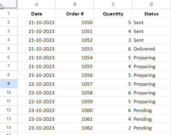
Sample Data
We used the following sample data in the Excel formula example above. We will use the same data in Google Sheets so that you can see how the SUMIFS with OR logical condition differs in Google Sheets and Excel.
SUMIFS with OR Condition in Google Sheets: REGEXMATCH
This approach offers several advantages. You do not need to use wildcards for partial matches separately, if any.
Additionally, you can make the SUMIFS function with OR logic case-sensitive.
Let me explain the logic behind using REGEXMATCH in SUMIFS, and then we will write the formula.
In the previous problem, specifying the criterion in the date column is straightforward because we don’t need to apply the OR logical test.
The challenge arises in the status column. Here, we need to test two conditions: “Sent” and “Delivered.”
Please refer to the screenshot below for the following REGEXMATCH array formula in cell E2:
=ARRAYFORMULA(REGEXMATCH(D2:D14,"Sent|Delivered"))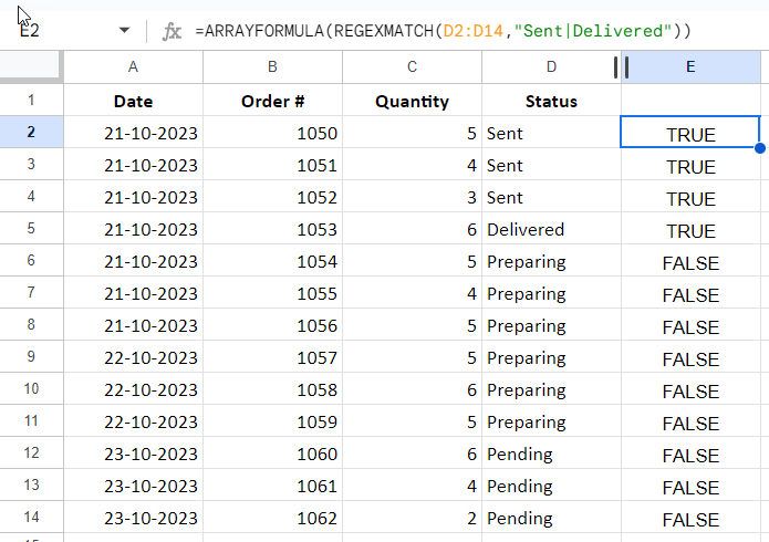
This formula will return an array of Boolean values.
Syntax of the REGEXMATCH Formula:
REGEXMATCH(text, regular_expression)If the value in the cell contains “Sent” or “Delivered,” the corresponding element in the array will be TRUE, indicating a match. If the cell does not contain either of these words, the element in the array will be FALSE, indicating no match.
In this case, the criteria are case-sensitive, and it’s a partial match. If you want an exact match, not a wildcard match, replace the regular expression "Sent|Delivered" with "^Sent$|^Delivered$".
If you want to make it case-insensitive but require an exact match, not a wildcard match, use "(?i)^Sent$|^Delivered$"
Now, here’s the multiple criteria SUMIFS formula with OR logic in Google Sheets:
=SUM(SUMIFS(C2:C14,A2:A14,DATE(2023,10,21),E2:E14,TRUE))We have replaced the status column, originally in the D2:D14 criteria range, with the result of the REGEXMATCH formula.
Note: You don’t need to use the helper column E2:E14. In SUMIFS, replace that range with the REGEXMATCH formula itself.
SUMIFS with OR Condition in Google Sheets: Lambda
Using MAP or BYROW lambda with SUMIFS is another way to handle SUMIFS with OR logic in Google Sheets.
Here is an example using MAP as per the sample data above:
=SUM(MAP({"Sent","Delivered"},LAMBDA(row, SUMIFS(C2:C14,A2:A14,DATE(2023,10,21),D2:D14,row))))This formula works as follows:
In this formula, we utilize the MAP function to iterate over the array {"Sent","Delivered"} and apply the lambda function to each element within this array.
The lambda function, defined as LAMBDA(row, SUMIFS(C2:C14, A2:A14, DATE(2023, 10, 21), D2:D14, row)), is a crucial part of the formula.
The row serves as the argument passed to the lambda function, representing either “Sent” or “Delivered.”
The MAP function essentially executes the lambda function twice, once with “Sent” and once with “Delivered” as the row argument, resulting in two values.
The SUM function aggregates the returned values, giving us the final sum of the results.
Wildcard Match
To use partial matches in SUMIFS with OR condition, use the asterisk (*) wildcard character.
For example, to match any word that contains “sent” or “delivered”, use the wildcards as follows:
{"*Sent*","*Delivered*"}The asterisk (*) wildcard character matches any sequence of characters, including zero characters.
In this case, the wildcards will match any word that contains the string “sent” or “delivered”, regardless of any other characters that may be present in the word.
Note: The formula is not case-sensitive.
Alternatives to SUMIFS with OR Condition in Google Sheets
If you are looking for a perfect solution to replace SUMIFS with OR criteria, then use QUERY.
The QUERY function can be used to perform a variety of tasks, including SUMIFS with OR criteria. There are several ways to do this, using either the logical OR operator or the Matches or Contains string comparison functions.
- Query with OR Logical Operator (Case Sensitive and Exact Match):
=QUERY(A2:D14,"select sum(C) where A=date '2023-10-21' and D='Sent' or D='Delivered' label sum(C)''")- Query with Matches String Comparison (Case Sensitive and Exact Match):
=QUERY(A2:D14,"select sum(C) where A=date '2023-10-21' and D matches 'Sent|Delivered' label sum(C)''")- Query with Contains String Comparison (Case Sensitive and Partial Match):
=QUERY(A2:D14,"select sum(C) where A=date '2023-10-21' and D contains 'Sent' or D contains 'Delivered' label sum(C)''")Notes:
- The default behavior of string comparison functions like Matches and Contains is case-sensitive. To make them case-insensitive, convert the strings to lowercase using the Lower function before comparing.
- The Contains string comparison function will match any string that contains the specified substring, regardless of its position in the string.
Conclusion
You may have observed that I hardcoded the criteria in all of the SUMIFS formulas with OR conditions above. You can use cell references instead. Please refer to the relevant functions in my function guide to learn more about criteria usage.
I hope you enjoyed this tutorial. Thanks for your time!


