To apply alternating colors (zebra striping) to visible rows, both Google Sheets and Excel offer built-in features and custom formula options:

The built-in alternating colors feature in Google Sheets provides seamless adaptation to filtered ranges when rows are hidden using Data > Filter, Slicer, or View > Grouping. However, manually hidden rows can disrupt the formatting.

We can also use a custom formula in conditional formatting in Google Sheets that offers a more dynamic and adaptable solution for visible rows, even when rows are manually hidden.

What about Excel?

In Excel, we can use the format as table feature, which conveniently applies alternating colors that adjust to any hidden rows but requires converting the data range into a table, which might not always be desirable.

Similar to Google Sheets, in Excel also, we can use a custom formula in conditional formatting. It provides an alternative method to achieve alternating colors for visible rows without table formatting.

In the following sections, we’ll explore both built-in and formula-based approaches in detail, starting with Google Sheets.

Purpose of Alternating Colors in Spreadsheets

Zebra striping is a design technique that offers several benefits in spreadsheets. Here are some of the most important ones:

1. Improves Readability: It enhances the readability of tabular data by providing visual separation between records (rows).
2. Facilitates Focus: Alternating colors reduce the chance of losing one’s place within a table, making it easier for users to focus on relevant information.
3. Highlights Patterns in Data: In scenarios such as payroll data, where start time is in one row and end time is in another, zebra striping helps in highlighting patterns.
4. Enhances Aesthetics: Zebra striping contributes to the overall aesthetics of a spreadsheet.

Applying Alternating Colors to Visible Rows in Google Sheets

As mentioned earlier, there are two approaches to applying alternating colors to visible rows in Google Sheets: a built-in feature and a conditional formatting approach.

The Built-in Alternating Colors Approach in Google Sheets

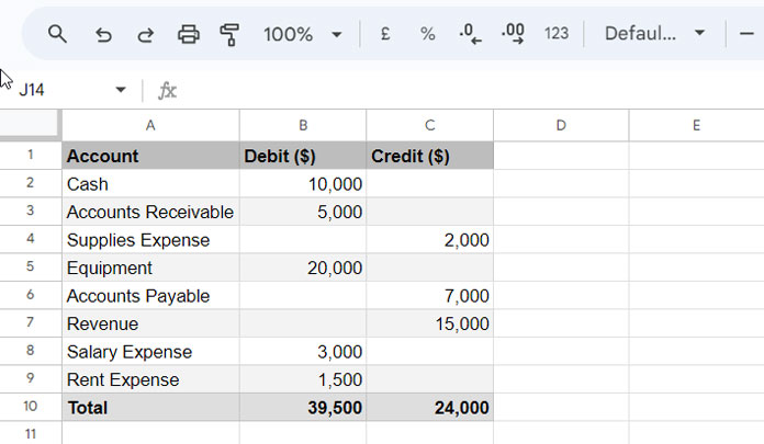
Assume you want to apply alternating colors to visible rows in the range A1:C10 in Google Sheets. Here are the steps to follow:

1. Select the range A1:C10.
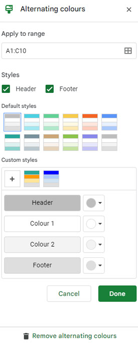
2. Click Format > Alternating colors.
3. On the sidebar panel, under “Styles,” check or uncheck the options “Header” and “Footer.” These options are useful when you have a header row in your table that contains field labels and a footer that contains totals or summary information.
4. You can choose different zebra striping styles as well as create custom styles.
5. To create a custom alternating color, click on the + button, select “Color1,” “Color2,” and click “Done.” If you have checked the “Header” and “Footer,” you will get the option to select custom colors for them too.

Important:

• It will retain the zebra striping pattern, even if you apply a filter to the range using Data > Filter, Data > Slicer, or View > Group. However, in a filtered range, if you undo an action (Edit > Undo or using the shortcuts Ctrl + Z in Windows and ⌘ + Z in Mac), the zebra striping will be a mess.
• If you manually hide rows using the “Hide” option in the context (right-click) menu, the zebra striping will not dynamically adjust to the remaining visible rows.

How do I remove the alternating colors applied to visible rows using the built-in feature in Google Sheets?

Click anywhere within the highlighted range and go to Format > Alternating colors. Then, click on “Remove alternating colors.”

The Formula Approach in Google Sheets

If you want to apply alternating colors that dynamically adjust to visible rows in Google Sheets, you can use my formula in conditional formatting.

It has no glitches that occur with the Undo action, as mentioned in the built-in approach. Also, it will respond to Data > Filter, Data > Slicer, View > Group, and Manual hiding of rows.

Prerequisites:

• Column Without Blank Cells: The formula relies on a column within your formatting range that has no blank cells. If necessary, create a helper column.
• Formula for Helper Column: =SEQUENCE(ROWS(A1:A10)) (replace A1:A10 with one of the column ranges from your actual formatting range). Enter this formula in the top cell of a blank column within or adjacent to your formatting range.

Note: Using a helper column is generally preferred, even if you have a column without blank cells in your formatting range. This is because inserting rows within the range can lead to blank cells, disrupting the formula’s accuracy. The SEQUENCE formula in the helper column dynamically adjusts to accommodate inserted rows, ensuring consistent formatting.

Conditional Formatting Formula:

=ISODD(SUBTOTAL(103, $A$1:$A1)) // Adjust for your column/helper column

Explanation:

• SUBTOTAL(103, $A$1:$A1): Calculates a running count within visible rows.
• ISODD(…): Determines if the count is odd, returning TRUE or FALSE for alternating formatting.

To apply zebra striping to visible rows, we need to apply this in conditional formatting. So the TRUE rows will be highlighted with our chosen fill color. Here is how to do that.

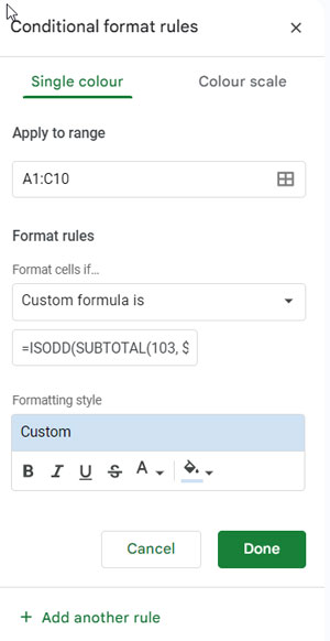
• Select the desired range (e.g., A1:C10).
• Navigate to Format > Conditional formatting.
• Verify the “Apply to range.”
• Choose “Custom formula is.”
• Paste the corrected formula, adjusting cell references if needed.
• Select a fill color under “Formatting style.”
• Click “Done.”

How to Remove Alternating (Visible) Row Color Highlighting in Google Sheets?

Click on any cell in the highlighted range.

Click on Format > Conditional formatting and remove the rule applied for the range A1:C10.

Applying Alternating Colors to Visible Rows in Excel

In Excel, we will use the built-in feature to apply alternating colors to visible rows first. Remember, while doing so, you will format the range as a table.

The Built-in Format as Table Approach in Excel

1. Select the range of cells, here A1:C10, that you want to apply zebra striping.
2. In the Home tab, under the Styles group, click Format as Table and select any zebra striping presets.
3. It will open the Create a Table dialog box. Check or uncheck “My Table has Headers” and click OK.

It has no glitches and will dynamically adjust the alternating row colors to any type of filtering. The only issue with this is that the created table.

To remove the alternating colors in Excel:

1. Click on any cell within the table.
2. Go to the Table Design tab.
3. Under the Table Styles group, click None.
4. Under the Tools group, click Convert to Range.
5. A confirmation dialog will appear asking if you want to convert the table to a normal range. Confirm by clicking Yes.

The Formula Approach in Excel

Similar to Google Sheets, we can use a formula within conditional formatting in Excel to apply alternating colors to visible rows. The prerequisites under The Formula Approach in Google Sheets apply here as well.

Here are the steps to follow:

Copy the following formula, which we used in Google Sheets:

=ISODD(SUBTOTAL(103, $A$1:$A1))

Select the range A1:C10.

Go to the Home tab > Styles group and click on Conditional Formatting > New Rule.

Click on “Use a formula to determine which cells to format” and paste the copied formula in the field below that.

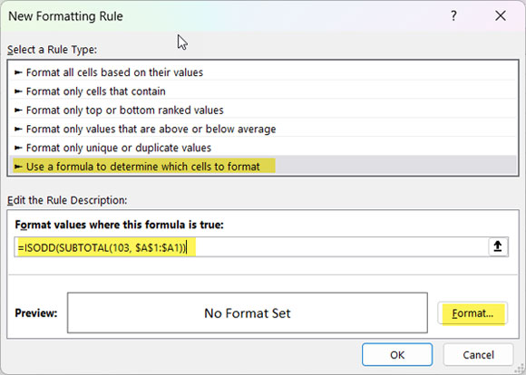
On the same dialog box, click Format. Then, within the opened Format Cells dialog box, select Fill and choose any color other than white. Click OK twice to close both the Format Cells and New Formatting Rule dialog boxes.

You have finished applying alternating colors to visible rows in Excel.

Note: To remove highlighting, select the range A1:C10, and click on Home > Conditional Formatting > Clear Rules > Clear Rules from Selected Cells.

Conclusion

Though Google Sheets and Excel have built-in features to apply alternating colors to filtered ranges or tables, both features are distinct.

In Excel, it creates a table and applies the formatting style, while Google Sheets merely applies a formatting style. Furthermore, in Google Sheets, manual hiding of rows and undoing a filter action can disrupt the zebra striping, which is not the case in Excel.

The format rules (formula-based zebra striping) behave similarly in both applications, although the approach to applying and removing them differs.

In short, use the formula-based approach in both spreadsheet applications if you want better control over alternating colors in visible rows.

Related:

• Highlight a Set of Alternate Rows in Google Sheets
• Highlight Every Alternate Set of N Columns In Google Sheets