We’ll explore various formula options for running counts in Google Sheets, starting with a non-array formula and moving to array formulas.
To return the running count of values in A2:A, use the following formula in cell B2 and drag it down as far as needed:
=IF(A2="", ,COUNTIF($A$2:A2, A2))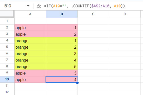
This formula follows the syntax: IF(logical_expression, value_if_true, value_if_false)
Here, the logical_expression is A2="", which checks if the cell is blank. If the expression evaluates to TRUE (meaning the cell is blank), the formula returns an empty string.
If the expression evaluates to FALSE (meaning the cell has a value), the formula executes the COUNTIF function.
COUNTIF($A$2:A2, A2) returns the count of the value up to the current row. The COUNTIF function follows the syntax: COUNTIF(range, criterion).
In this formula, the range expands as we drag the formula down because it uses a mixed reference. The starting point ($A$2) is fixed, but the endpoint (A2) adjusts based on the row where the formula is applied. For example, in row #10, the range will be $A$2:A10 (mixed reference), and the criterion will be A10 (relative reference).
Running Count Array Formula Options in Google Sheets
If you prefer an array formula that sits in the first cell and expands down for a running count, there are three main options based on:
- COUNTIFS
- SORT and MATCH
- MAP Lambda Function
We will explore all these options in the examples below, but I typically prefer the COUNTIFS method for its simplicity and efficiency.
Option 1: Using COUNTIFS for Running Count
The following formula in cell B2 will return the running count of the values in A2:A:
=ArrayFormula(IF(A2:A="",,COUNTIFS(A2:A, A2:A, ROW(A2:A), "<="&ROW(A2:A))))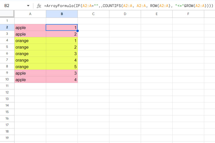
When using this formula, replace A2:A with the cell range for which you want the running count.
Formula Breakdown for Option 1
We use the ARRAYFORMULA function because we want to apply the ROW, COUNTIF, and IF functions across an entire array, not just a single cell.
The purpose of the IF logical test is to return a blank in rows where the cell value is empty.
This running count array formula is essentially a COUNTIFS array formula.
Syntax: COUNTIFS(criteria_range1, criterion1, [criteria_range2, …], [criterion2, …])
If we use the formula with just two arguments, criteria_range1 and criterion1, it would be:
=ArrayFormula(IF(A2:A="",,COUNTIFS(A2:A, A2:A)))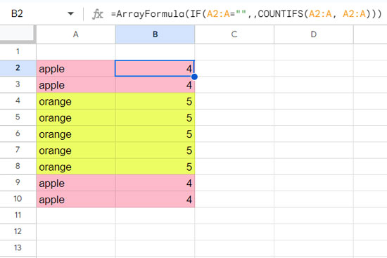
This would return the total count of values in the entire range.
For example, if the value “Orange” repeats 5 times, the formula will assign “5” to each occurrence. However, we want the running count of occurrences, such as a sequence from 1 to 5.
The second criteria range, ROW(A2:A), and the criterion "<="&ROW(A2:A) make the difference. This part ensures the formula counts the values up to the current row in each row by checking if the row numbers are less than or equal to the current row number.
Option 2: Using SORT and MATCH for Running Count
This method is a bit more complex for calculating a running count in Google Sheets. Let’s first apply the formula in cell B2 for the range A2:A, and then go over the explanation:
=IFNA(
   SORT(
      SEQUENCE(ROWS(A2:A), 1, 2)-MATCH(SORT(A2:A), SORT(A2:A), 0),
      SORT(SEQUENCE(ROWS(A2:A), 1, 2), A2:A, 1), 1
   )
)
While this option isn’t as widely used as the COUNTIFS method, it still works effectively. Now, let’s break down how it works.
Formula Breakdown for Option 2
To calculate a running count in a sorted range (note that all our formulas are designed to work regardless of sorting), use the following formula in cell B2:
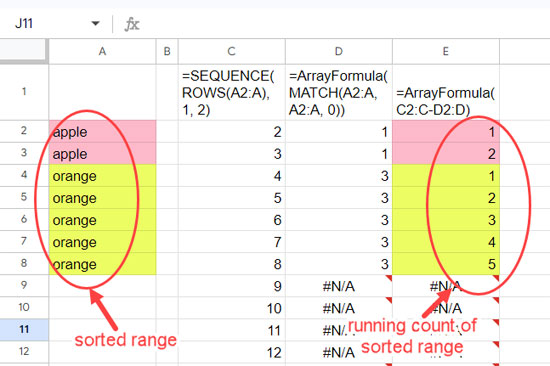
=ArrayFormula(IFNA(SEQUENCE(ROWS(A2:A), 1, 2)-MATCH(A2:A, A2:A, 0)))In this formula, SEQUENCE(ROWS(A2:A), 1, 2) generates a sequence of numbers from 2 to the last row in the range.
MATCH(A2:A, A2:A, 0) returns the relative position of each item in the range. The first occurrence gets a 1, and all subsequent occurrences get the same number.
Subtracting the result of MATCH from the sequence numbers gives the running count.
To adapt this formula for a range regardless of sorting, modify it as follows:
SORT(seq_start_at_2 - match_of_sorted_range, seq_start_at_2_sorted_by_range, true)There are two parts to this:
- In this version, MATCH is applied to a sorted version of the range. The generic formula part is
seq_start_at_2 - match_of_sorted_range, whereseq_start_at_2isSEQUENCE(ROWS(A2:A), 1, 2)andmatch_of_sorted_rangeisMATCH(SORT(A2:A), SORT(A2:A), 0). - The following part returns the sequence numbers sorted by the range:
SORT(SEQUENCE(ROWS(A2:A), 1, 2), A2:A, TRUE).
SORT(part_1, part_2, 1) will yield the running count of occurrences.
The IFNA function handles any #N/A errors resulting from MATCH in empty rows.
Option 3: Running Count with MAP Lambda Function
At the beginning of this tutorial, we explored a drag-down formula for running count. We can enhance this formula using the MAP and LAMBDA functions as follows:
=MAP(A2:A, LAMBDA(currentItem, IF(currentItem="",,COUNTIF(A2:currentItem, currentItem))))Enter this formula in cell B2 to return the cumulative count of occurrences of values in A2:A.
The MAP function iterates over each value in the array A2:A and returns new values by applying a custom function defined using LAMBDA.
In this case, the LAMBDA function is LAMBDA(currentItem, IF(currentItem="",,COUNTIF(A2:currentItem, currentItem))), where currentItem represents the current element in the array as specified in MAP.
So, the COUNTIF range will be A2:A2, A2:A3, A2:A4, … in each row, and the criterion will be A2, A3, A4, … in each row. This is because the endpoint of the range is represented by currentItem, which is also used as the criterion.


Hi Prashanth,
I’m currently working on setting up a rolling sequential number for purchase orders. I’ve developed a macro that automatically clears specific contents within the order.
I’m attempting to write a formula that, when I click the “New Order” button, deletes the desired data and advances the number to the next sequential value on the order form. However, I’m encountering difficulty in ensuring that the purchase order number updates to the next available sequential number.
Thanks Scotty
I’m trying to find a running count of the number of times a customer has ordered, with their phone number being the customer identifier.
The issue here is that my data input software is glitchy, and sometimes a duplicate order shows up in my file.
How it is:
Order ID | Customer Phone # | Running Count (formula column)
123 | 111111111 | 1
123 | 111111111 | 2
456 | 222222222 | 1
Customer 111111111 only placed one order, but their duplicate order makes it seem as if they’ve ordered twice.
Fortunately, I have order IDs, which are unique to every order placed.
I was wondering, if there is some way to add to the formula where the duplicate orders are ignored?
How I want it to look like:
Order ID | Customer Phone # | Running Count (formula column)
123 | 111111111 | 1
123 | 111111111 |
456 | 222222222 | 1
My purpose is to get accurate re-ordering insights. I’ve stuck on this for a long time. Any help would be highly appreciated!
Hi, Fatima,
I clearly understand the problem. You can solve it effectively.
If the running count of IDs is equal to 1, rerun the running count of phone numbers, else blank.
This formula in cell C2 may return your expected result if the above data is in A1:B, where A1:B1 contain field labels.
=ArrayFormula(if(countifs(row(A2:A),"<="&row(A2:A),A2:A,A2:A)=1, countifs(row(A2:A),"<="&row(A2:A),B2:B,B2:B),) )
As a side note, we can use COUNTIFS also in an unsorted list.
Hello,
I have a google sheet with Dates in Column A, File Codes in Column B example:
20 January 2020 | D87
18 February 2020 | D87
20 February 2020 | C49
01 March 2020 | D51
31 March 2020 | D51
I want to generate File names according to the Financial Year in Column C.
Example:
20 January 2020 | D87 | A-20D87001
18 February 2020 | D87 | A-20D87002
20 February 2020 | C49 | A-20C49001
01 March 2020 | D51 | A-20D51001
31 March 2020 | D51| A-20D51002
I’m stuck at the last digit. What formula should I apply to get running counts?
Hi, Kiran Suresh,
I don’t clearly understand your question. You may try this first. If it doesn’t work as expected, share the URL of your sample sheet in your reply below.
Assume the first row contain titles (column names), and you want the file names in C2:C.
In D2, insert the following running count array formula and see the result.
=ArrayFormula(if(len(B2:B),text(COUNTIFS(year(A2:A)&B2:B,year(A2:A)&B2:B,row(B2:B),"<="&row(B2:B)),"000"),))Hello,
I tried using the above formula, but I think I did something wrong. So I’m sharing the URL of the sample spreadsheet:
– URL of the sample sheet removed by admin –
Hi, Kiran Suresh,
The issue was in the year part. I have used column G to specify the corresponding financial year and used that column in my new formula.
={"File Name";ArrayFormula(if(len(C3:C),"A"&right(G3:G,2)&C3:C&text(COUNTIFS(G3:G&C3:C,G3:G&C3:C,row(C3:C),"<="&row(C3:C)),"000"),))}
Please check your sheet for my new tab named test_infoinspired.
Wow!.. Thank you so much Sir..!! Thanks a lot.. 🙂
ROW(A2:A),"<="&ROW(A2:A)Could you please explain this part more? I understand that it creates a counter for each item in a list, but how does it work.
Thanks
Hi, Ryan,
It’s actually a simple logical test but ‘difficult’ to explain.
The logical test returns TRUE up to the current row from the first row in the range.
E.g.
A2 – TRUE
A2 – TRUE, A3 – TRUE
A2 – TRUE, A3 – TRUE, A4 – TRUE
… and so on.
Hi Prashanth,
I have a table with 2 columns:
Col1 – list of names and class (e.g. “John History”, “Billy Math”)
Col2 – list of grades
What I need to be able to do is rank the scores for each student.
Example of data:
John History | 60
John Math | 50
John Algebra | 70
John Physics | 20
Billy History | 65
Billy Math | 20
Billy Algebra | 90
Billy Physics | 100
Can you please assist?
Hi, Valo,
I assume the names are in A2:A (A1 contains the label “Name”) and B2:B contains the scores (B1 contains the label “Scores”).
Solution:
I have three solutions.
The formula for cell C2 using the RANK function:
=ArrayFormula(IFNA(rank(B2:B,B2:B,1)))If two persons have the same score, the formula will return the same rank.
Eg.:
Both John Physics and Billy Math scored 20. So their rank will be 1.
Since the next rank of the person will be 3, not 2.
The formula for cell D2 using the RANK.AVG function:
=ArrayFormula(IFNA(RANK.AVG(B2:B,B2:B,1)))It follows the same above ranking principles, except the rank will be 1.5 (average).
The formula for cell E2 using a Custom Formula:
=ArrayFormula(IFNA(vlookup(A2:A,{index(sort(A2:B,2,1),0,1),ArrayFormula(if(len(B2:B),match(index(sort(A2:B,2,1),0,2),
unique(index(sort(A2:B,2,1),0,2)),0),))},2,0)))
Here the ranks of John Physics and Billy Math will be 1. But the next rank of the person will be 2, not 3.
Pick the formula that is suitable for you.
I have a Google Sheets with last names in column B and first names in column C.
I would like to have a count in column E of each time a combination of last and first name appear together.
I was able to get the count working using
=countifs(B:B, B2,C:C, C2)However, I would 2nd and 3rd times the name combinations appear to demonstrate 2 and 3 instead of all showing the current count.
Hi, Daniel,
You can combine the first and last names and use the running count as below in E2.
=ARRAYFORMULA(if(len(B2:B),COUNTIFS(B2:B&C2:C,B2:B&C2:C,ROW(A2:A),"<="&ROW(A2:A)),))This formula will populate the running count of the last and first names in E2:E. So, before inserting the formula, make E2:E blank.
Thanks a lot, I was stuck on finding the cumulative count of all items in the lists. This helped me a lot.
Hi Prashanth,
I am trying to do a running count of a single item in google sheets, similar to your “Running Count of Single Item – Non-Array Formula” example.
I want the sequential count to be in column A, and I want it to count all the sections in column B that end with the words “blog post”.
Ex:
Column (A) | Column (B)
1 | blah blah blog post.
– | test string.
2 | learning google sheets blog post.
3 | need help with the sheets blog post.
– | chapter 8 notes.
I pasted
=if(B2:B="*blog post*",COUNTIFS(B$2:B,"*blog post"),)into A2, but nothing is showing up. Where am I going wrong?Hi, Sohail Merchant,
There are two issues in your partial matching running count formula.
1. The wildcard use
B2:B="*blog post*"is wrong.2. Inside the COUNTIFS (you can also use COUNTIF) instead of
B$2:Byou must useB$2:B2.Here is the proper formula to use in your case.
=iferror(if(search("blog post",B2:B)>0,COUNTIFS(B$2:B2,"*blog post*"),))How do I go about making this formula dynamic? Do I turn it into an array by using “arrayformula”? When I tried using array formula it just made every item that ends with ‘blog post’ the same number.
Hi, Sohail Merchant,
In partial matching, using ArrayFormula alone won’t work. You may please try this one.
=ARRAYFORMULA(IFERROR(if(search("blog post",B2:B10)>0=TRUE,COUNTIFS(search("blog post",B2:B10)>0,search("blog post",B2:B10)>0,ROW(B2:B10),"<="&ROW(B2:B10)),)))=ARRAYFORMULA(COUNTIFS(A2:A10,A2:A10,ROW(A2:A10),"<="&ROW(A2:A10)))can handle even unsorted list.Good catch!
Thanks.