The COUNTIFS array formula in Google Sheets lets you count values in a range based on multiple criteria, all while handling results dynamically.
Unlike SUMIFS, which behaves more consistently, COUNTIFS can spill down (expand results automatically) in most cases, but there are situations where it won’t expand as expected.
In this tutorial, I’ll show you how to overcome these COUNTIFS array formula issues using other functions like LAMBDA or REGEX in combination with COUNTIFS. You’ll also learn the standard use of the COUNTIFS function itself.
COUNTIFS Function Syntax in Google Sheets
Mastering the syntax is the first step to using COUNTIFS effectively.
Syntax:
COUNTIFS(criteria_range1, criterion1, [criteria_range2, …], [criterion2, …])Arguments:
- criteria_range1: The first range to evaluate against criterion1.
- criterion1: The condition that determines which cells in
criteria_range1are counted. It can be a number, text, expression, date, or a cell reference. - criteria_range2, criterion2: Optional, repeatable additional ranges and criteria.
Before exploring COUNTIFS array formula in Google Sheets, let’s go through some examples of basic non-array COUNTIFS usage.
Basic COUNTIFS Formulas with Multiple Criteria
Here are a few examples of COUNTIFS with different types of criteria. These are standard (non-array) formulas but demonstrate how COUNTIFS works.
Make a copy of my sample sheet to follow along (click the button below).
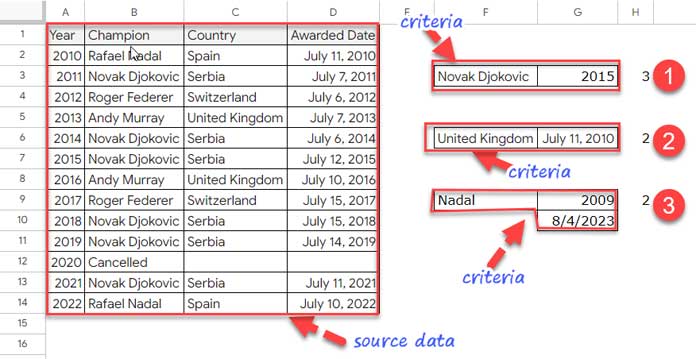
1. COUNTIFS with Text and Number Criteria
In H3:
=COUNTIFS(B2:B, F3, A2:A, ">"&G3)This formula counts how many titles “Novak Djokovic” won after 2015.
Hardcoded version:
=COUNTIFS(B2:B, "Novak Djokovic", A2:A, ">2015")2. COUNTIFS with Text and Date Criteria
In H6:
=COUNTIFS(C2:C, F6, D2:D, ">="&G6)This formula returns the number of titles where column C equals “United Kingdom” and column D is on or after July 11, 2010.
Hardcoded:
=COUNTIFS(C2:C, "United Kingdom", D2:D, ">="&DATE(2010, 7, 11))3. COUNTIFS with Wildcards, Numbers, and Dates
In H9:
=COUNTIFS(B2:B, "*"&F9, A2:A, ">"&G9, A2:A, "<"&G10)This counts Nadal’s titles from 2010 to the date in G10.
Hardcoded with wildcard and TODAY:
=COUNTIFS(B2:B, "*Nadal", A2:A, ">"&2009, A2:A,"<"&TODAY())The wildcard * ensures that partial matches, such as finding ‘Nadal’ within ‘Rafael Nadal,’ are included.
COUNTIFS Array Formula and Natural Expansion
The real strength of the COUNTIFS array formula in Google Sheets is its ability to expand results automatically. For example, if new rows are added, the formula can spill down results without dragging.
However, sometimes COUNTIFS won’t expand correctly. Let’s see examples.
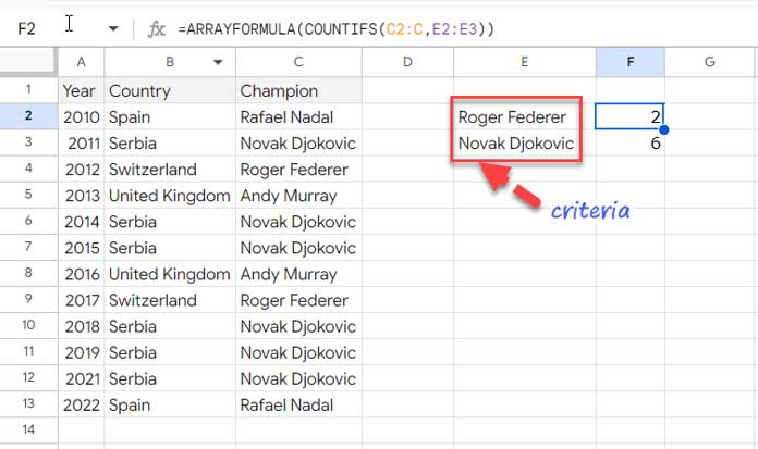
Example 1: Basic COUNTIFS Spill-Down
In F2:
=ARRAYFORMULA(COUNTIFS(C2:C, E2:E3))This applies COUNTIFS across multiple criteria in E2:E3, returning counts automatically.
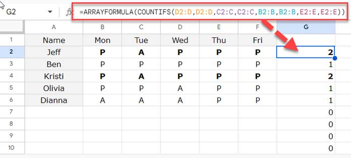
Example 2: Identifying Duplicate Patterns
=ARRAYFORMULA(COUNTIFS(D2:D, D2:D, C2:C, C2:C, B2:B, B2:B, E2:E, E2:E))This checks if rows (like attendance records) repeat across employees. If the result is greater than 1, it means a duplicate pattern exists.
To remove zeros that appear from blank or unmatched rows, wrap the COUNTIFS formula with LET + IF:
=ARRAYFORMULA(
  LET(result, COUNTIFS(D2:D, D2:D, C2:C, C2:C, B2:B, B2:B, E2:E, E2:E),
  IF(result=0,, result))
)
In this formula, LET assigns the COUNTIFS result to a named variable result, making the formula easier to read and maintain. The IF statement then replaces any zero values with blanks, so your output only shows meaningful counts.
COUNTIFS Array Formula with OR Conditions
Sometimes you need “this OR that” criteria. COUNTIFS doesn’t natively support OR, but we can work around it.
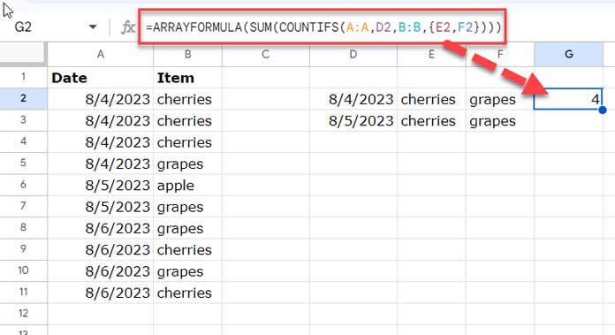
Example 1: OR in a Single Column
=ARRAYFORMULA(SUM(COUNTIFS(A:A, D2, B:B, {E2, F2})))This counts purchases of cherries or grapes on a given date.
For spill-down across multiple rows, use LAMBDA + MAP:
=MAP(
  D2:D3, E2:E3, F2:F3,
  LAMBDA(x, y, z,
    ARRAYFORMULA(SUM(COUNTIFS(A:A, x, B:B, {y, z})))
  )
)
Explanation:
This formula applies the COUNTIFS logic row by row using MAP and LAMBDA. For each row in D2:D3, E2:E3, and F2:F3, it calculates the COUNTIFS result and spills it automatically, so you don’t need to drag the formula down.
When to use this:
Use MAP + LAMBDA when your criteria generate multiple values per row (such as OR conditions like {y, z}) and you need to aggregate them with functions like SUM or COUNT. MAP handles each row independently, ensuring that array-valued criteria inside COUNTIFS are properly evaluated and aggregated into a single result per row.
Example 2: OR Across Multiple Columns
Using REGEXREPLACE simplifies multi-column OR conditions:
=ARRAYFORMULA(
   COUNTIFS(
      REGEXREPLACE(C:C, "(?i)apple|orange", "A"), "A",
      REGEXREPLACE(D:D, "(?i)In-stock|Ordered", "B"), "B",
      B:B, F2:F3
   )
)
This counts apples or oranges with status In-stock or Ordered on specific dates.
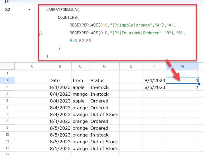
Explanation:
REGEXREPLACE converts multiple textual OR conditions in each column into a single placeholder (e.g., “A” or “B”), which COUNTIFS can then count efficiently. ARRAYFORMULA allows the formula to spill across multiple rows.
When to use this:
Use REGEXREPLACE + COUNTIFS when you have OR conditions in multiple columns and want a single COUNTIFS formula to handle all criteria. This is especially useful when each column can contain multiple possible values that need to be counted together.
Conclusion
The COUNTIFS array formula in Google Sheets is powerful for handling multiple criteria, dynamic expansions, and even OR conditions with the right helpers like LAMBDA and REGEX.
I’ve walked you through from basic COUNTIFS usage to advanced array formula techniques.
For more, check out:
Master these, and you’ll be able to handle any COUNTIFS scenario confidently.


