COUNTIFS with multiple criteria in the same range refers to applying more than one condition in a single column for counting in Google Sheets.
COUNTIFS is used to count a range based on multiple criteria. This usually involves conditions from more than one column.
However, sometimes conditions need to be tested in the same column along with conditions in other columns.
The following syntax clearly specifies “criterion1”, “criterion2” in separate ranges, not “criterion1”, “criterion2”, … in the same range (criteria_range1):
COUNTIFS(criteria_range1, criterion1, [criteria_range2, …], [criterion2, …])This tutorial will guide you on the proper way to use multiple criteria in the same range in COUNTIFS in Google Sheets.
COUNTIFS with Multiple Criteria in the Same Range
Assume you have a list of fruits in the range A2:B where A2:A contains the date of receipt and B2:B contains fruit names. Let’s apply COUNTIFS with multiple criteria in this range.
Single Column:
Assume you want to count the fruits Apple, Orange, and Mango in that range.
So, the criteria_range1 will be B2:B, and criterion1 will be the array {"Apple", "Orange", "Mango"}.
Here is the correct approach to use multiple criteria in the same range in COUNTIFS in Google Sheets:
=ArrayFormula(
   COUNTIFS(
      ((B2:B="Apple")+(B2:B="Mango")+(B2:B="Orange")), 1
   )
)
Where:
criteria_range1:((B2:B="Apple")+(B2:B="Mango")+(B2:B="Orange"))criterion1:1
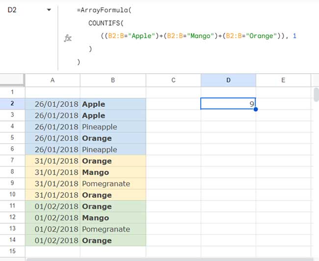
Explanation:
This formula works by evaluating each condition (B2:B="Apple", B2:B="Mango", B2:B="Orange") individually. Each condition results in TRUE or FALSE (which is equivalent to 1 or 0 in a numeric context). The + operator sums these results for each cell in B2:B.
If a cell matches any of the criteria, it results in 1 (TRUE), otherwise 0 (FALSE).
Using ARRAYFORMULA ensures this evaluation is applied across the entire range.
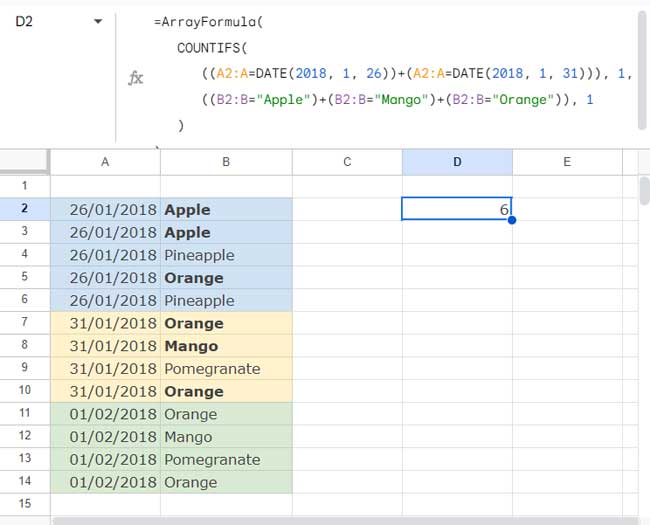
Multiple Columns:
You can follow the same approach when you want to apply multiple criteria in the same range but in two different columns.
Problem:
Find the count of Apple, Orange, and Mango received on 26/01/2018 and 31/01/2018.
Formula:
=ArrayFormula(
   COUNTIFS(
      ((A2:A=DATE(2018, 1, 26))+(A2:A=DATE(2018, 1, 31))), 1,
      ((B2:B="Apple")+(B2:B="Mango")+(B2:B="Orange")), 1
   )
)
Where:
criteria_range1:((A2:A=DATE(2018, 1, 26))+(A2:A=DATE(2018, 1, 31)))criterion1: 1criteria_range2:((B2:B="Apple")+(B2:B="Mango")+(B2:B="Orange"))criterion2:1
Additional Notes:
In the above formulas, I’ve hardcoded the criteria within the formula. You can replace them with cell references as well.
For example, if you specify the criteria Apple, Mango, and Orange in C2:C4, then the formula will be as follows:
=ArrayFormula(
   COUNTIFS(((B2:B=C2)+(B2:B=C3)+(B2:B=C4)), 1)
)
If you have several criteria in a range, consider using functions that use pattern matching, as explained in my tutorial here: OR in Multiple Columns in COUNTIFS in Google Sheets.
COUNTIFS with Multiple Criteria in the Same Range and QUERY Alternative
QUERY is an alternative function for handling multiple criteria within the same range, whether for counting or summing purposes.
So, we can use it to replace COUNTIFS or SUMIFS with multiple criteria in the same ranges in Google Sheets.
In the above sample data, we can use the following QUERY formula to count the occurrence of Apples, Oranges, and Mangos in B2:B:
=QUERY(A2:B, "SELECT COUNT(A) WHERE B='Apple' OR B='Mango' OR B='Orange'")To count the above fruits received on either 26/01/2018 or 31/01/2018, use the following QUERY:
=QUERY(A2:B, "SELECT COUNT(A) WHERE (B='Apple' OR B='Mango' OR B='Orange') AND (A=DATE '2018-01-26' OR A=DATE '2018-01-31')")Note: The above formulas are case-sensitive.
Please check my function guide to learn about QUERY and also search this site for more information.
Resources
- Google Sheets: COUNTIFS with Not Equal to in Infinite Ranges
- COUNTIFS in a Time Range in Google Sheets [Date and Time Column]
- Not Blank as a Condition in COUNTIFS in Google Sheets
- COUNTIF | COUNTIFS Excluding Hidden Rows in Google Sheets
- How To Use COUNTIF or COUNTIFS In Merged Cells In Google Sheets
- Varying Array Sizes in COUNTIFS in Google Sheets
- OR in COUNTIFS in Either of the Columns in Google Sheets
- COUNTIFS with ISBETWEEN in Google Sheets
- Counting XLOOKUP Results with COUNTIFS in Excel and Google Sheets


I hope you can help. I’m trying to count the number of TRUE values (checked boxes) in a given range of cells based on a range of dates defined in two other cells.
And to top it off, if there is no defined “end date,” can I get it to use today as the end date instead?
I was trying with
=COUNTIFS(C10:DD10, true, $C$4:$DD$4>=G62,$C$4:$DD$4<=H62,$C$4:$DD$4<=TODAY())but that returns an error that says COUNTIFS expects all arguments after position 2 to be in pairs.I tried adding an IF statement in there, but that didn’t work, either.
Can you help? Thanks!
Hi, Chris Slater,
This may work.
=countifs(C10:10,true,C4:4,">="&G62,C4:4,"<="&if(H62,H62,today()))Brilliant! It works. Thank you!
Is it possible to choose one of such criteria?
If I select Apple in a drop-down, the only value that should appear is the count of Apple.
If I leave the drop-down blank, then the values that should appear are the count of all/specified fruits/values.
I use the following formula:
=ARRAYFORMULA(SUM(COUNTIFS(A:A;{"D1";{"APPLE";"ORANGE";"POMEGRANATES"}};B:B;"1/6/2022")))*D1 = Dropdown for Apple/Orange/Pineapple/Pomegranates
Here is the demo: – URL removed by the Admin –
Hi, Raffi,
I understood your points. You want to COUNTIFS with multiple criteria or a single criterion based on the drop-down in cell D1.
This will do that.
=ARRAYFORMULA(SUM(COUNTIFS(A:A,if(len(D1),D1,{"APPLE";"ORANGE";"PINEAPPLE";"POMEGRANATES"}),B:B,"1/6/2022")))And as per your Locale (spreadsheet settings), use it as,
=ARRAYFORMULA(SUM(COUNTIFS(A:A;if(len(D1);D1;{"APPLE";"ORANGE";"PINEAPPLE";"POMEGRANATES"});B:B;"1/6/2022")))I want to use this but it’s not working can someone help…
=if(F5="","", COUNTIFS($W5:$BW5,{"Present","Present H"})/COUNTIFS($W$4:$BW$4,"*****"))Hi, Rashid Qureshi,
Try this.
=ArrayFormula(IFERROR(if(F5="","", SUM(COUNTIFS($W5:$BW5,{"Present","Present H"}))/COUNTIFS($W$4:$BW$4,"*****"))))
=SUM(COUNTIFS(D2:D50,{"Sr.";"Jr."},C2:C50,{"M","M/A"}))This is my excel formula, but when moved to Google Sheets, it doesn’t work.
I have ready to insert ArrayFormula as noted in the example above.
=ArrayFormula(SUM(COUNTIFS(D2:D50,{"Sr.";"Jr."},C2:C50,{"M","M/A"})))However, this does not work. Please provide any simple suggestions.
Hi, Chris,
In Google Sheets, you can try different combinations. Here is one.
Exact Match:
=counta(filter(C2:C50,regexmatch(C2:C50,"^M$|^M\/A$")*regexmatch(D2:D50,"^Sr\.$|^Jr\.$")))
Partial Match:
=counta(filter(C2:C50,regexmatch(C2:C50,"M|M\/A")*regexmatch(D2:D50,"Sr\.|Jr\.")))
I am trying to get a count if for Tuesdays that have a greater value than 90 in cells M2:M145 in google sheets. What am I doing wrong here?
=(COUNTIFS('POSITIVE CLOSE'!A2:A145,"Tue",M2:M145,">90"))Hi, Omid D Danielpour,
Your formula seems correct to me.
If you have dates in A2:A145 formatted as day names, try the below formula.
=ArrayFormula(COUNTIFS(text('POSITIVE CLOSE'!A2:A145,"ddd"),"Tue",M2:M145,">90"))Also, check the locale settings of your Sheet.
Hi Prashanth,
I am trying to count a series of data in a column, say M2:M145.
I want it to count all instances where values were positive in a series of 3 times or more.
Meaning, If M2, M3, M4 were positive in value, it would count as 1.
If M6, M7, and M8 were positive, count it and add up to 2, etc.
If M9 and M10 were positive but M11 was negative, it would not add and move on through the column.
Hi, Omid D Danielpour,
What would be the count if M5 was positive?
Hi, Prashanth,
Thanks for the follow-up.
If M5 in that series is positive as well, the count would remain unchanged, and it would count it as 1 still.
It’s looking to identify three or more uninterrupted occurrences of positive values.
If M6, M7, and M8 were positive, that series would still count as just 1.
Hi, Omid D Danielpour,
I have tested the below formula, and it seemed to work.
=ArrayFormula(countif(
countif(filter(lookup(row(M1:M145),if({-1;M2:M145}<0,row(M1:M145))),{-1;M2:M145}>=0),
unique(filter(lookup(row(M1:M145),if({-1;M2:M145}<0,row(M1:M145))),{-1;M2:M145}>=0)))
,">=3")
)
You can try it. If you want a formula explanation as a tutorial, please let me know.
This is a very useful post! I am wondering if there would be a way to use it to simplify my sample spreadsheet.
I am collecting dates, types, and names at different sessions, and I am compiling the number of times per week that each person leading a session. Right now I am using COUNTIFS with conditions on the date, type, and name, but I need to add a new COUNTIFS (with the same date and type conditions) for each person leading. Would there be a simpler way to do this?
Thank you for your support!
Hi, Nikita,
I could partially achieve that with FLATTEN, and then a Query multiple column Pivot.
Please see the tab “Sheet1 – II” in your shared sheet for the formula.
Hi Prashanth,
Thank you for your quick reply, really appreciate it! That is quite an interesting way to do it, I have a lot more to learn. Thanks again 🙂
Very useful !!
Hi Prashanth,
Please help me to use the below formula in google sheets. In Excel, I am using;
=SUM(COUNTIFS(D1,A4,D4,{"Booked","WIP","Pending","PFC Pending","PFC In Progress","PFC Completed","QC Correction","Client Correction","QC","QC WIP","QC Pending","1 - QC Done","1 - QC WIP","Send for Approval","Hold","Hold - 1 QC","Hold - 2 QC","Uploaded","QC Passed","Dispatch Ready","Approved","Dispatch WIP","Dispatch Needed"}))Hi, Pavan,
Wrap your above formula with the ArrayFormula function as per the below syntax.
=ArrayFormula(your_above_formula)But for me, it seems the arguments are not properly inputted in your Countifs.
COUNTIFS(criteria_range1, criterion1, [criteria_range2, …], [criterion2, …])As per your formula, the cells D1 and D4 are criteria_range1 and criterira_range2. Is that correct?
Sharing a sample/mockup sheet will be helpful to understand the issue.
Is it possible to multiply the COUNTIF statements for a range of data?
=countif('title'!A10:A20,"Help")But then what I want to do is if “Help” shows up, then be able to multiply it by the value that would be entered into B10:B20.
Hope this makes sense. Thanks
Hi, Derek.
I guess you want to count “Help” in A10:A20, sum corresponding values in B10:B20, and then multiply both the outputs. If so, there are several ways.
Here are a few of them that I may use in such a scenario in Google Sheets.
Using Countif and Sumif:
=countif(title!A10:A20,"Help")*sumif(title!A10:A20,"Help",title!B10:B20)
Using two Filter formulas, Count, and Sum:
=COUNT(filter(title!B10:B20,title!A10:A20="Help"))*sum(filter(title!B10:B20,title!A10:A20="Help"))
Using Query:
=query(title!A10:B20,"Select count(A)*sum(B) where A ='Help' label count(A)*sum(B)''",0)
Hi Prashanth,
If I say this correctly,
If cell A1 not empty, and if one or more cells in B1:E1 is not empty, how can I count in F1 result as = 1?
Thank you.
Try this formula, please.
=if(ArrayFormula(SUM(len(B1:E1)*len(A1)))>0,1,)Hi, Prashanth,
Thank you for your response, have a great day.
Thank You.
Hi,
I tried using the formula but function not working.
I need the count of the words specified in the formula. kindly help Thanks.
Hi, Bindu,
I have added the following Query on your Sheet.
=query({$A$1:A},"Select Count(Col1) where lower(Col1) contains '"&lower(C9)&"' label Count(Col1)''")If you want an explanation of this formula, please let me know.
Best,
Hi Guys,
Can anyone help me out?
How can I execute the below formula?
=COUNTIFS(Sheet1!$AK:$AK,$A23,Sheet1!$AJ:$AJ,"NO",Sheet1!$S:$S,"To be Scheduled Later - Customer","To be Scheduled Later - Rupeek")Hi, Mohan,
I guess there are multiple conditions to be evaluated in column S. Then the COUNTIFS formula would be something like;
=sum(ArrayFormula(COUNTIFS(Sheet1!$AK1:$AK,$A23,Sheet1!$AJ1:$AJ,"NO",Sheet1!$S1:$S,{"To be Scheduled Later - Customer",
"To be Scheduled Later - Rupeek"})))
Best,
I don’t know when it was added but there is now a
=COUNTUNIQUEIFS()function that does exactly this.Hi, Ryan,
Thanks a ton for this info!
I think it’s a newly added function in Sheets.
Hi Prashanth, I am trying to have more than 2 Countif arguments. Below is the formula
=COUNTIFS('Master Attrition 2018'!B:B,'World Wide - 2018'!$C$5,=Countif('Master Attrition 2018'!P:P,'Master Attrition 2018'!"*Remort*")'Master Attrition 2018'!H:H,'World Wide - 2018'!B7). – Its not workingThe reason I wanted to use the 3rd argument because I want to have the part of the data from each of those cells (Remort – from Remort -NJ, Remort-SFO, Remort-NY, Remort-WC). Thanks
Hi, Ramana,
Can you prepare a demo Sheet and share here?
Hi, I’m trying to get the sum of this to Countifs.
=countifs('Masterfile PV Validation'!G:G,A64,'Masterfile PV Validation'!P:P,"Yes")=countifs('Masterfile PV Validation'!G:G,A64,'Masterfile PV Validation'!S:S,"Yes")
Hi, Erolle,
You can try this.
=countifs('Masterfile PV Validation'!G:G,A64,'Masterfile PV Validation'!P:P,"Yes")+countifs('Masterfile PV Validation'!G:G,A64,'Masterfile PV Validation'!S:S,"Yes")
Here is the Sumproduct alternative.
=sumproduct('Masterfile PV Validation'!G1:G=A64,'Masterfile PV Validation'!P1:P="Yes")+sumproduct('Masterfile PV Validation'!G1:G=A64,'Masterfile PV Validation'!S1:S="Yes")In a second thought, I find you may want to count column G if the values in both column P and S is Yes. If so, give this formula a try.
=sumproduct('Masterfile PV Validation'!G1:G=A64,'Masterfile PV Validation'!P1:P="Yes",'Masterfile PV Validation'!S1:S="Yes")Hope this helps.
Hi Prashanth,
Thanks for the well explained post…really helpful