In this Google Sheets tutorial, I will explain how to use COUNTIF or COUNTIFS to exclude hidden or filtered rows.
COUNTIF can only handle one criterion, so we cannot use it to exclude hidden rows in Google Sheets. We need to specify at least two conditions for the conditional count: one condition for the desired value and one condition to exclude hidden rows.
Therefore, we must use COUNTIFS, even if we only want to apply one criterion. To exclude hidden rows in a conditional count, we will use COUNTIFS, not COUNTIF.
Sample Data:
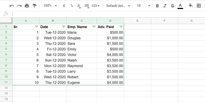
The sample data in columns A:D contain serial numbers, date, employee name, and advance paid, respectively.
I have filtered the dataset by selecting the range A1:D11 and then clicking the Data menu > Create a filter.
Now, let’s make the necessary settings for COUNTIFS to exclude hidden rows in Google Sheets. Before that, let’s see how to count cells excluding hidden rows (not conditional count).
Getting Started with COUNTIFS Excluding Hidden Rows in Google Sheets
Do you know how many ways there are to hide a row or multiple rows in Google Sheets?
As far as I know, in Google Sheets, there are four built-in ways to hide rows:
- Select the rows you want to hide and right-click, then select “Hide rows 6 – 7” (or whatever the row numbers are).
- Click on the Filter drop-down in cell C1 (we have already filtered our sample data), uncheck “Victor” and “Ralph,” and click the OK button. (This is the method we are following.)
- Select the rows you want to hide and right-click, then select “View more row actions” and “Group rows 6 – 7.” (Or whatever the row numbers are.) Then toggle the + or – button.
- Use the Slicer (
Datamenu >Add a Slicer).
Once you have hidden the rows using any of the above methods, insert the following SUBTOTAL formula in cell C13:
=SUBTOTAL(103,C2:C11)This will return 8.
The actual count is 10, but the count excluding hidden rows is 8. This is because SUBTOTAL treats the count of the values in the hidden rows as 0.
We will use the same Subtotal method in COUNTIFS excluding hidden rows in Google Sheets, because COUNTIF or COUNTIFS has no such feature to exclude the hidden rows.
How to COUNTIFS Excluding Hidden Rows in Google Sheets
For our purpose, we can use SUBTOTAL in two ways:
- In a helper column range.
- In an array formula using MAP Lambda.
Assume you want to get the count of values in D2:D where the values are greater than or equal to 3000. This is the regular COUNTIF formula:
=COUNTIF(D2:D11,">=3000")Here is the COUNTIFS alternative:
=COUNTIFS(D2:D11,">=3000")Let’s convert this COUNTIFS formula to exclude hidden rows:
Syntax of the COUNTIFS Function:
COUNTIFS(criteria_range1, criterion1, [criteria_range2, …], [criterion2, …])We have used criteria_range1 in the formula which is D2:D11. We should make a SUBTOTAL test on this column. If there are two columns (criteria_range1 and criteria_range2), then you can choose one of the columns for the test.
The SUBTOTAL test can be an array or non-array formula. Let’s see that below in the COUNTIFS excluding hidden or filtered-out row examples.
1. Helper Column Approach
Please follow these steps:
- Unhide the hidden rows, if any (we have hidden two rows in the previous example, right?).
- In cell E2, insert the following SUBTOTAL formula and copy and paste it down to cell E11, or drag the E2 fill handle down to cell E11:
=SUBTOTAL(103,D2)
Here is the syntax of the SUBTOTAL function:
SUBTOTAL(function_code, range1, [range2, …])Where:
103is the function code of the COUNTA function.range1isD2, the first cell to test in D2:D11, which is the column used in the COUNTIFS above.
In cell F2, insert the following COUNTIFS formula:
=COUNTIFS(D2:D11,">=3000",E2:E11,"=1")Where:
D2:D11is thecriteria_range1.">=3000"is thecriterion1.E2:E11is thecriteria_range2."=1"is thecriterion2.
This COUNTIFS will exclude hidden rows in the result.
How is this possible?
The SUBTOTAL function returns 0 in hidden rows and 1 in visible rows. We have used this as a criterion in COUNTIFS to exclude hidden row values in the result.
2. COUNTIFS Excluding Hidden Rows without a Helper Column
SUBTOTAL is one of the Google Sheets functions that does not expand on its own or with the help of the ARRAYFORMULA function. This is where the LAMBDA function comes in.
If you don’t want to drag the SUBTOTAL function in cell E2 down, you can use the following MAP formula in cell E2:
=MAP(D2:D11, LAMBDA(row, SUBTOTAL(103, row)))Note: You must remove all the values in E2:E11, even in the hidden rows, before entering this formula in cell E2. If the previous SUBTOTAL non-array formulas are in one of the cells in this range, this will return a #REF! error.
Here is the syntax of the MAP lambda helper function:
MAP(array1, lambda(name, formula_expression))Where:
D2:D11isarray1.rowis the name ofarray1.SUBTOTAL(103, row)is theformula_expression.
The MAP function iterates over each value in the array1 to return a SUBTOTAL array result.
Can we use this formula within the COUNTIFS instead of using it in cell E2?
Yes! Just replace E2:E11 in the the helper column-based COUNTIFS formula with the above MAP formula, like this:
=COUNTIFS(D2:D11, ">=3000", MAP(C2:C11, LAMBDA(row, SUBTOTAL(103, row))), "=1")You can use the above formula to COUNTIFS excluding hidden rows in Google Sheets.
Resources
Here are some related resources.
- Google Sheets Query Hidden Row Handling with Virtual Helper Column.
- SUMIF Excluding Hidden Rows in Google Sheets [Without Helper Column].
- How to Omit Hidden or Filtered out Values in Sum [Google Doc Spreadsheet].
- Vlookup Skips Hidden Rows in Google Sheets – Formula Example.
- Check Whether a Row Is Hidden and Highlight the Row above It in Google Sheets.
- Insert Sequential Numbers Skipping Hidden | Filtered Rows in Google Sheets.
- Subtotal with Condition in Google Sheets [Step by Step Guide].
- Grouping and Subtotal in Google Sheets and Excel.
- How to Subtotal Up to the First Blank Cell in a Column in Google Sheets.
- Subtotal Function With Conditions in Excel and Google Sheets.


Hi,
Thanks so much for the help, I really appreciate it! Makes a lot more sense now. I’ll try in the future to use more the Array Formulas for sure 🙂
Another question if you have a thought on this: do you think that using a similar formula it could be possible to know how many tests are done every month (using the date columns and the options column)? I will try to do something with what you suggested 🙂
Thanks again, have a great day
Hi Prashanth,
Thanks for the article, it was super helpful! I managed to work something out using the formula you provided:
=countifs(G10:G176, "Federica B", byrow(B10:B176, lambda(r, subtotal(103, r))), "=1")It’s working well, but I’m still facing a very weird issue. Without applying any filtering options, the formula displays 7. When I apply one filter, it shows 1. So far, so good. But when I switch from one tab to another, the 1 “blinks” back to 7, even though the filtering option remains the same.
I know it’s a bit unclear, but I was wondering if you had any ideas why it would be doing that. Thanks a lot!
Hi Eric T,
“… But when I switch from one tab to another, the 1 “blinks” back to 7, even though the filtering option remains the same.”
I haven’t faced any such issue. If you want, you can share a copy of your sheet with me. Please remove any sensitive or personal information.
As a side note, I’ve just updated this post to replace BYROW with MAP. But that doesn’t affect the result.
Hi Prashanth,
I submitted a reply two days ago with a link to the sheet, but it seems like it did not go through the moderation review. Please let me know if I can share it with you in another way.
Thanks for your help!
Eric
Hi Eric,
I’ve seen the sheet, but I can’t find where to look for the specific COUNTIFS hidden row issue. Additionally, you have several non-array formulas that make it difficult for a third person to read.
Please share the sheet again if you have specific details about where to look and what the issue is. This will save me a lot of time and effort.
Hi Prashanth,
Thanks for the reply. I apologize for the previous sheet, which was a bit difficult to read. I have attached an updated version, which I hope is easier to understand, along with the following explanation:
On the tab
SS_Count, there is a Pivot table (which takes its data from theRaw_Datasheet) with a Slicer to filter on theSeasoncolumn.On the tab
Import, in cell D4, there is a long COUNTIFS formula. This formula counts the number of times each name appears in the table, multiplied by the number of versions. Although this formula may not be the most efficient, it is the only way I could find to perform the counting, and it is working correctly.The goal is that when using the Slicer to filter on different seasons, the number of times each name appears in the table should automatically update (excluding the rows that are hidden by the filtering). However, for some reason, the formula is not adjusting properly.
I hope this makes it easier for a third person to understand the file and how it works. Thank you very much for your help.
Link to updated spreadsheet: [removed by admin]
Hi Eric T,
Thanks. I understand now 🙂
In short, you want to sum (not count) the
Optionscolumn in theSS_Countsheet for the names in theImportsheet that match the names in theSS_Counttester columns (Tester W1,Tester W2,Tester W3, etc.). The formula should be responsive to filtering applied in theSS_Countsheet.I don’t know why you haven’t used my SUBTOTAL array formula to generate the helper column. In cell
SS_count!A8, I have inserted the following formula, which will return 1 in visible rows and 0 in hidden rows. You can find an explanation of the formula in my SUBTOTAL function tutorial (function guide):=VSTACK("Helper",MAP(C9:C,LAMBDA(row,SUBTOTAL(103,row))))If you replace your SLICER with Data > Create a filter, the COUNTIFS seems to work as expected. I think the issue is that you are applying COUNTIFS excluding hidden rows in a Pivot Table.
Actually, your COUNTIFS is not very useful or reader-friendly. It is very long and error-prone, even though you have done it very carefully.
Instead of copying and pasting that already long COUNTIFS into every row, you can use my following SIMPLE array formula in cell Import!I3:
=VSTACK("% of tests",MAP(C4:C, LAMBDA(row, SUM(BYCOL(SS_Count!G9:Z,LAMBDA(col, SUMIFS(SS_Count!C9:C,SS_Count!A9:A,1,col,row)))))))
You need SUMIFS, not COUNTIFS.
Please check your shared sheet for the formulas.
Hello: I am using the following formula:
=COUNTIFS('TAB 1'!$E:$E,B$6,'TAB 1'!$F:$F,$A7)The range ‘TAB 1’A1:F1000’ has filters in the header rows.
How do I get the above formula to consider ONLY the data that remains visible when I use the filters?
Hi, George G,
I thought I had well explained the same in the tutorial. Here is the formula for you.
=COUNTIFS('Tab 1'!$E:$E,B$6,'Tab 1'!$F:$F,$A7,byrow('Tab 1'!$F:$F,lambda(r, subtotal(103,r))),1)