The core purpose of the SUBTOTAL function in Google Sheets is to work with filtered and grouped data.
It can replace the AVERAGE, COUNT, COUNTA, MAX, MIN, PRODUCT, STDEV, STDEVP, SUM, VAR, and VARP functions when you want only to include visible rows in aggregations. These eleven aggregation functions cannot distinguish between visible and hidden rows, but SUBTOTAL can.
How can a single function replace 11 other functions?
By using function codes.
Since SUBTOTAL can handle 11 aggregation functions, you can use it in dynamic dashboards to switch from sum to average or other aggregations using a drop-down list.
The SUBTOTAL function in Google Sheets has another feature that you may admire if you handle a very large volume of data.
Assume you have a column with several rows of data and several group totals using the SUM function. Placing a grand total at the last row in that column can be time-consuming because you need to go to each subtotal row and add them using the + operator.
However, SUBTOTAL makes this task simple. This is a feature that I have used extensively.
Another feature of SUBTOTAL is that we can use it with LAMBDA functions to create a virtual helper column, which we can then use in other functions such as COUNTIF and QUERY to make them work with visible rows.
The four purposes of the SUBTOTAL function at a glance:
- Calculate subtotals and grand totals in a list.
- To work with filtered and grouped data.
- To switch between functions in dynamic dashboards.
- To create a virtual helper column for handling filtered rows in other functions using LAMBDA functions.
Syntax and Arguments
Syntax of the SUBTOTAL function in Google Sheets:
SUBTOTAL(function_code, range1, [range2, …])Arguments:
function_code: A numeric code that specifies the type of calculation you want to perform.
Each function has two codes and you can use either of them if you have no hidden rows. But they do differ in handling hidden rows.
| Function | Exclude rows hidden by filter or slicer | Exclude rows hidden by filter, slicer, right-click, or row grouping |
| AVERAGE | 1 | 101 |
| COUNT | 2 | 102 |
| COUNTA | 3 | 103 |
| MAX | 4 | 104 |
| MIN | 5 | 105 |
| PRODUCT | 6 | 106 |
| STDEV | 7 | 107 |
| STDEVP | 8 | 108 |
| SUM | 9 | 109 |
| VAR | 10 | 110 |
| VARP | 11 | 111 |
range1: The first range over which to calculate a subtotal..
range2, …: (optional) Additional ranges over which to calculate subtotals.
Related: Google Sheets Function Numbers: A Comprehensive Guide
How to Use the SUBTOTAL Function to Calculate Subtotals and a Grand Total in a Column
We usually insert subtotals when we have multiple sorted categories in a table.
For example, let’s say you have a billing statement sorted by customer names in column B. There are three customers named A, B, and C.
To sum each customer’s invoice amount in column C, you can use the SUBTOTAL function instead of SUM.
=SUBTOTAL(9,C2:C5) // total invoice amount for customer A
=SUBTOTAL(9,C8:C12) // total invoice amount for customer B
=SUBTOTAL(9,C15:C19) // total invoice amount for customer C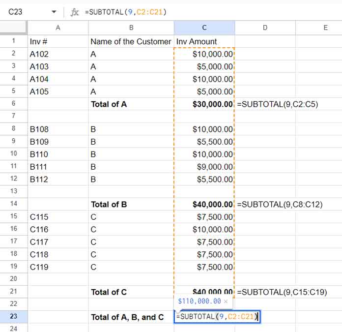
The benefit of using the SUBTOTAL function instead of SUM in this example is that the SUBTOTAL function will exclude the results of the SUBTOTAL formulas in C6, C14, and C21 when calculating the grand total (total of customers A, B, and C) in C23.
=SUBTOTAL(9,C2:C21)If you use the SUM function, you will need to use either of the following functions to calculate the grand total, which can be error-prone and tedious if you have a large volume of data:
=SUM(C6,C14,C21)
=C6+C14+C21
SUBTOTAL Function in Google Sheets to Calculate Subtotals for Visible Rows
In this test, we will use Filter, Slicer, Right-Click Hide, and Grouping to see how the SUBTOTAL function works with visible data.
We will use the function codes 2 and 102 for the test. These are the function numbers representing the COUNT function.
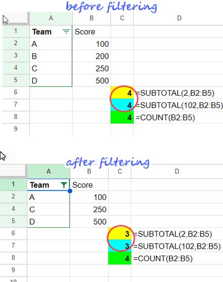
In cell C6, insert the following formula:
=SUBTOTAL(2,B2:B5)In cell C7, insert the following formula:
=SUBTOTAL(102,B2:B5)And insert the following COUNT formula in cell C8:
=COUNT(B2:B5)All of these formulas will return 4 if all the cells in the range B2:B5 are non-blanks and they are non-empty.
Now, let’s see how these formulas react to visible rows.
1. “Create a filter” Test
Select the range A1:A5, then go to Data > Filter. This will place a filter drop-down in cell A1.
Click on the filter drop-down menu icon in cell A1, uncheck “C”, and click OK.
The SUBTOTAL functions in cells C6 and C7 will return 3, while the COUNT function in cell C8 will still return 4.
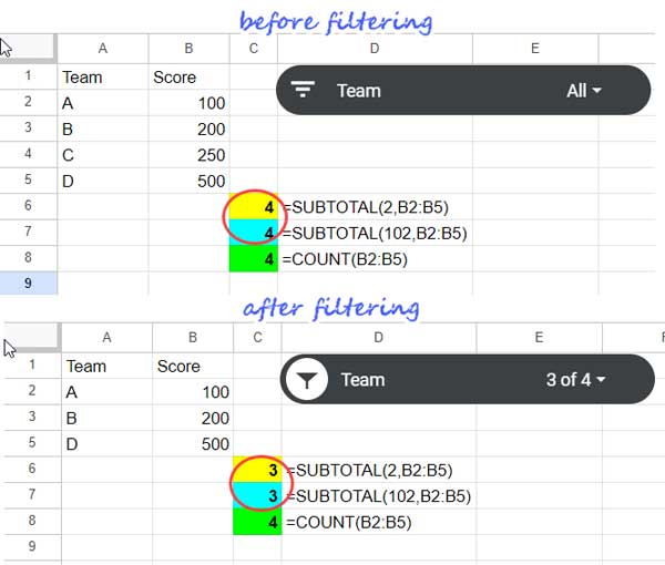
2. “Add a Slicer” Test
When using Slicers, the SUBTOTAL functions, and the COUNT function will work similarly to the “Create a filter” test above.
To create a Slicer, select the range A2:B5 and then go to Data > Add a Slicer.
In the Slicer dialog box on the sidebar panel, under “Column”, select “Team”.
Then, click on the filter drop-down on the Slicer, uncheck “C”, and click OK.
The SUBTOTAL functions in cells C6 and C7 will return 3, while the COUNT function in cell C8 will still return 4.
3. Right-click and “Hide row” Test
Here you will see the difference between function code 2 and function code 102.
Right-click on row 4 and click “Hide row”.
The SUBTOTAL formula in cell C6, which uses function number 2, and the COUNT formula in cell C8 will not have any effect, while the SUBTOTAL formula in cell C7, which uses function code 102, will only count the visible rows.
4. Group Rows Test
The values in grouped rows are included or excluded in the SUBTOTAL function similar to the values in right-click hidden rows. Function codes 1 to 11 will include them (hidden rows) in the calculation, while function codes 101 to 111 will exclude them.
To test this, select row numbers 2 and 3 to group them. To do this, click on row 2, press the Shift key, and click on row 3. Then, click on View > Groups > Group rows 2 – 3. Click on the minus button to collapse the group.
The =SUBTOTAL(102, B2:B5) formula will return the count of visible rows, while the =SUBTOTAL(2, B2:B5) formula will return the count of all rows.
SUBTOTAL Function to Switch Between Functions in Dynamic Dashboards
Before we get to the core part of this topic, let’s first create a Data validation drop-down menu in cell E2.
First, enter all the function names supported in SUBTOTAL in the range I1:I11 so that we can quickly create a drop-down menu.
Select cell E2 and then go to Insert > Data validation. In the Data validation dialog box, under Criteria, select “List from a range”. In the next field, select the data range I1:I11 and then click OK.
Now to the sample data for the test.
We have meeting minutes dates in column A and the number of participants in column B.
To get the total, average, min, max, and count of participants without using the SUBTOTAL function in Google Sheets, we would need to use five formulas:
=SUM(B2:B)
=AVERAGE(B2:B)
=MIN(B2:B)
=MAX(B2:B)
=COUNT(B2:B)
How do we dynamically switch from one function to another using the SUBTOTAL function in Google Sheets?
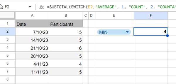
We have a drop-down in cell E2 that contains the names of all the functions we want to use.
Now use the following SWITCH function to return the function code based on the function selected in cell E2:
=SWITCH(E2,"AVERAGE", 1, "COUNT", 2, "COUNTA", 3, "MAX", 4, "MIN", 5, "PRODUCT", 6, "STDEV", 7, "STDEVP", 8, "SUM", 9, "VAR", 10,"VARP",11)Now use this formula as the function_code argument in the SUBTOTAL function and the range1 is B2:B:
=SUBTOTAL(SWITCH(E2,"AVERAGE", 1, "COUNT", 2, "COUNTA", 3, "MAX", 4, "MIN", 5, "PRODUCT", 6, "STDEV", 7, "STDEVP", 8, "SUM", 9, "VAR", 10,"VARP",11),B2:B)This will switch functions based on the function name selected in cell E2.
SUBTOTAL Array Formula in Google Sheets
Do we ever need to expand the SUBTOTAL function or any other aggregation functions? Yes. For example, when we want to subtotal multiple columns, we may need to use multiple SUBTOTAL formulas.
In the following example, I have copied the SUBTOTAL formula in B9 to C9, D9, and E9.
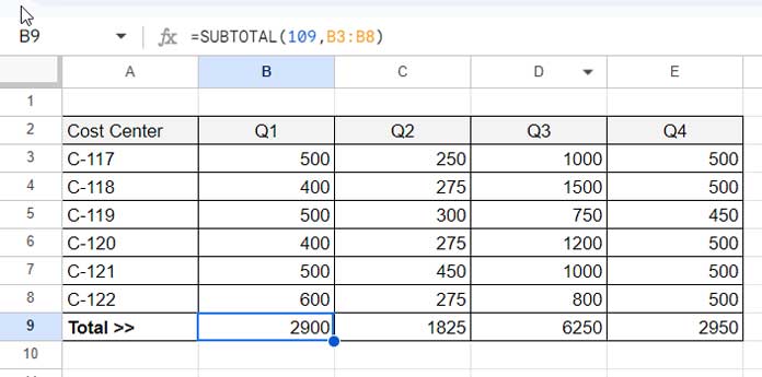
Using the BYCOL function, we can expand the SUBTOTAL formula in cell B9 to cells C9, D9, and E9.
=BYCOL(B3:E8,LAMBDA(col,SUBTOTAL(109,col)))The above formula uses the BYCOL function to apply the SUBTOTAL function to each column in the range B3:E8.
The BYCOL function takes two arguments:
- The first argument is the range of cells to apply the function. In this case, the range is B3:E8.
- The second argument is a function that takes a column as input and returns a value. In this case, the function is
LAMBDA(col,SUBTOTAL(109,col)).
The BYCOL function will apply the SUBTOTAL function to each column in the range B3:E8, and return a horizontal array of the results.
We can use this feature of the SUBTOTAL function to create a virtual helper column. Here’s how.
Virtual Helper Column Using SUBTOTAL Function in Google Sheets
I’ll first explain the purpose of creating a virtual helper column using the SUBTOTAL function in Google Sheets. Then, we’ll create one.
In the above example, how do we return the count of values in Q1 that are greater than 400?
You would use the following COUNTIFS formula:
=COUNTIFS(B3:B8,">400")However, this formula will not return the correct result if rows in the range are hidden.
To make the formula respond to hidden rows, we can use a SUBTOTAL helper column. We need to expand a SUBTOTAL formula down for this, not across, so we will use the MAP lambda function.
The data for Q1 is in the range B3:B8, so the virtual helper column must be based on it. Use function number 3 or 103, which is equal to COUNTA, pointing to the first cell in this range, which is B3.
=SUBTOTAL(3,B3:B9)Expand this formula down using the MAP lambda function as follows:
=MAP(B3:B8, LAMBDA(row,SUBTOTAL(3,row)))This formula will return 1 in visible rows and 0 in hidden as well as blank rows.
Now, let’s use this as the virtual helper column in the above COUNTIFS formula:
=COUNTIFS(B3:B8,">400",MAP(B3:B8, LAMBDA(row,SUBTOTAL(3,row))),1)This will count the values in visible rows in Q1 that are greater than 400.
Note: The BYROW lambda function can be used in place of the MAP lambda function to create a SUBTOTAL virtual column.
Similar: COUNTIF | COUNTIFS Excluding Hidden Rows in Google Sheets
Conclusion
As you have seen, the SUBTOTAL function is one of the most versatile functions in Google Sheets. It is designed to work with vertical data sets. Therefore, you can use it to insert subtotals in columns, exclude or include hidden rows, and calculate a grand total.
However, the SUBTOTAL function’s capability is limited when it comes to horizontal data sets. You can still use it to calculate subtotals and a grand total in a row, but it will not respond to hidden columns.


