How to Use the MAP Function in Google Sheets

The MAP function in Google Sheets lets you map each value in one or more arrays to a new value by applying a LAMBDA function.

As far as I know, it’s the only LAMBDA helper function (LHF) in Google Sheets that supports multiple arrays as input.

So naturally, it allows multiple name arguments within the LAMBDA.

For example, if you want to use three arrays individually in your MAP formula, you must specify name1, name2, and name3 within the LAMBDA.

Other LAMBDA helper functions (LHFs) like BYCOL, BYROW, SCAN, and REDUCE work with a single input array or range, applying a transformation row-by-row, column-by-column, or cumulatively.

In contrast, MAKEARRAY generates a new array from scratch by taking a specified number of rows and columns, then applying a LAMBDA function to determine the value for each cell based on its row and column index.

Table of Contents

MAP Function Syntax and Arguments in Google Sheets

Syntax:

MAP(array1, [array2, ...], LAMBDA)

Where:

array1 – The first array or range to be mapped.
array2, … – Additional arrays or ranges (optional).
LAMBDA – A lambda function containing name arguments (one per array) and a formula expression that defines how to transform each set of values.

LAMBDA Syntax in Google Sheets

LAMBDA([name, ...], formula_expression)(function_call, ...)

Note: The part in parentheses at the end is only needed when testing the LAMBDA function directly in a cell — that is, when using it on its own.

We can think of the syntax for the MAP function in Google Sheets as:

MAP(array1, ..., LAMBDA(name1, ..., formula_expression))

Step-by-Step: Using the MAP Function in Google Sheets

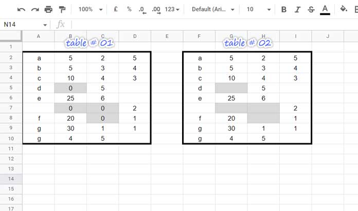
Without further ado, let’s look at an example. Check out the two tables in the screenshot below:

Table #1 contains sample data
Table #2 is the expected output (where 0 is replaced with blank)

Google Sheets example showing MAP function replacing 0s with blank in a single array

MAP Function Example – Single Array

Let’s say you want to use the MAP function in Google Sheets to transform each value in Table #1 and replace 0 with a blank. Here’s how to build the formula step-by-step:

Step 1: IF Logical Test (Standard Formula)

Enter this in cell F2:

=IF(A2=0, "", A2)

Step 2: Convert to a LAMBDA

=LAMBDA(v, IF(v=0, "", v))(A2)

The yellow-highlighted part (function call) is only for testing and is not needed in MAP.

Step 3: MAP Formula

=MAP(A2:D10, LAMBDA(v, IF(v=0, "", v)))

Here:

A2:D10 is the array
v is the name argument inside LAMBDA

Because we’re only mapping one array, we need just one name.

MAP Function Examples in Google Sheets

1. MAP Function to Expand Logical Tests (AND, OR)

Let’s say you want to check whether the values in A2:C2 are all equal:

=AND(A2=B2, A2=C2, B2=C2)

Trying to expand this across multiple rows using ARRAYFORMULA like below won’t work as expected:

=ARRAYFORMULA(AND(A2:A6=B2:B6, A2:A6=C2:C6, B2:B6=C2:C6))

It will return TRUE or FALSE (a single output).

But with the MAP function in Google Sheets, it’s straightforward to expand the result.

Even though you can achieve the same without MAP using multiplication logic:

=ARRAYFORMULA((A2:A6=B2:B6)*(A2:A6=C2:C6)*(B2:B6=C2:C6))

…it’s cleaner and more readable with MAP.

How the Formula Works Step-by-Step

1. Regular AND Logic:

=AND(A2=B2, A2=C2, B2=C2)

2. Convert to LAMBDA:

=LAMBDA(a, b, c, AND(a=b, a=c, b=c))(A2, B2, C2)

3. MAP Formula:

=MAP(A2:A6, B2:B6, C2:C6, LAMBDA(a, b, c, AND(a=b, a=c, b=c)))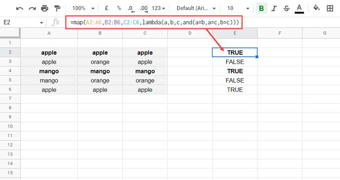

Output of MAP formula in Google Sheets applying AND logic across rows to check if values are equal

2. MAP with FILTER Function

Say you have a table of delivery records:

A2:A → Item name
B2:B → Location
C2:C → Quantity

You want to filter items that are either “Gravel 10–20 mm” or “Cobble Stone” and where the location is “Location 1”.

Here’s how to use the MAP function in Google Sheets for that:

=FILTER(A2:C, MAP(A2:A, B2:B, LAMBDA(a, b, AND(OR(a="Gravel 10-20 mm", a="Cobble Stone"), b="Location 1"))))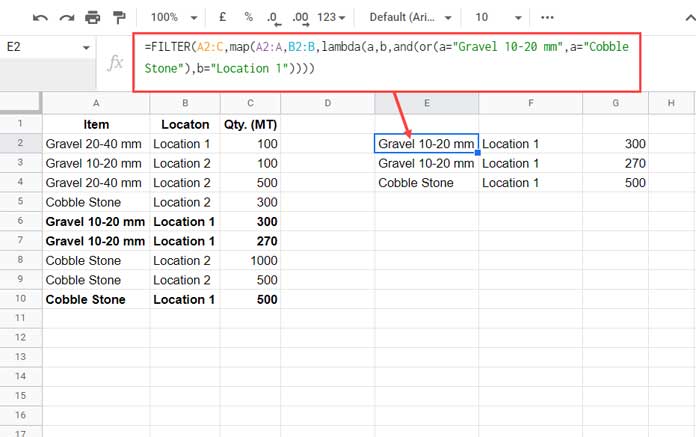

Google Sheets table filtered using MAP and LAMBDA to return specific items based on multiple conditions

How the MAP + FILTER Formula Works

Regular condition:

=AND(OR(A2="Gravel 10-20 mm", A2="Cobble Stone"), B2="Location 1")

Converted to LAMBDA:

=LAMBDA(a, b, AND(OR(a="Gravel 10-20 mm", a="Cobble Stone"), b="Location 1"))(A2, B2)

MAP expansion:

=MAP(A2:A, B2:B, LAMBDA(a, b, AND(OR(a="Gravel 10-20 mm", a="Cobble Stone"), b="Location 1")))

Used inside FILTER:

=FILTER(A2:C, [map_formula_output])

3. MAP with ISDATE

By default, ISDATE(A2:A) returns TRUE only if all values are dates. But what if you want to test each one individually?

Use MAP like this:

=MAP(A2:A, LAMBDA(dt, ISDATE(dt)))

This formula returns TRUE where the value is a date, and FALSE otherwise — row by row.

FAQs

I want to work on each row in a 2D array, not each element. Does MAP work?
No. In that case, use BYROW. For working with each column, use BYCOL.

MAP is cleaner. Should I replace traditional array formulas with MAP?
Only if it improves clarity or flexibility. While MAP is powerful, it can be resource-intensive on large datasets. Stick to traditional formulas when they get the job done efficiently.

Can I replace MAP with BYROW or BYCOL?
Yes — if you’re working with a one-dimensional array:

Use BYROW for vertical (column) arrays
Use BYCOL for horizontal (row) arrays

So don’t get confused if you see those in place of MAP in other formulas.