The AND logical function works with arrays in two ways in Google Sheets: it can return a single output or expanded results.

If you want to evaluate all values in an array and return TRUE or FALSE when they meet all conditions, you can apply the AND function with the ARRAYFORMULA.

If you want to use the AND function in an array to test if any conditions apply individually in each row, use AND with the MAP and LAMBDA functions. There is also a popular alternative using the logical * operator.

Let’s look at examples of using the AND function in arrays in Google Sheets.

Using the AND Logical Function in Arrays for a Single Output

The following formula tests whether all the values in the range B2:B12 fall between 50 and 100, returning TRUE or FALSE:

=ArrayFormula(AND(B2:B12>50, B2:B12<100))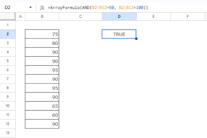

This type of ARRAYFORMULA application is useful when you want to check whether all the test scores fall within the specified limits.

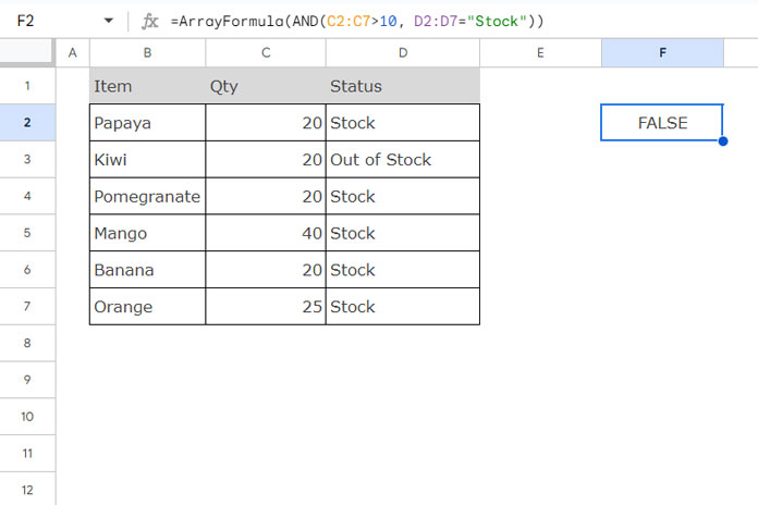
Here is another scenario where we test whether all the values in C2:C7 are greater than 10 and the values in D2:D7 are “Stock”:

=ArrayFormula(AND(C2:C7>10, D2:D7="Stock"))

This helps us verify that we have sufficient quantities in stock.

I hope these two examples help you understand the use of the AND logical function in arrays to get a single Boolean output.

Using the AND Logical Function in Arrays for Expanded Results

In both of the above examples, the AND function helps us determine whether the conditions are met. If the conditions are not met, we cannot identify the specific rows where they are not satisfied. This is where the following solutions become useful, as they allow us to expand the results for better clarity.

We can use the MAP function to expand the AND function results or use the * operator as an alternative to the AND function to expand the results.

Let’s take the second example above and apply the AND logical function to return expanded results in the arrays.

Using the Multiplication (*) Operator as an Alternative

The following formula in cell E2 will return 0 (FALSE) or 1 (TRUE) in the range E2:E7:

=ArrayFormula((C2:C7>10)*(D2:D7="Stock"))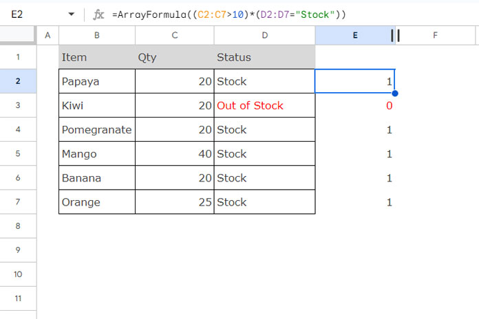

This formula works as follows:

• =ArrayFormula(C2:C7>10) // returns an array of TRUE or FALSE
• =ArrayFormula(D2:D7="Stock") // returns an array of TRUE or FALSE

In Google Sheets, the Boolean TRUE is equal to 1 and FALSE is equal to 0.

When you multiply these results (two arrays), the output is 1 if both conditions are met (TRUE * TRUE) and 0 if any condition is not met (FALSE * FALSE, FALSE * TRUE, TRUE * FALSE).

This is the logic behind using the alternative AND operator in an array for expanded results.

Using the MAP Lambda Functon

Instead of the above formula, you can also use the following MAP LAMBDA function in cell E2:

=MAP(C2:C7, D2:D7, LAMBDA(value1, value2, AND(value1>10, value2="Stock")))

This may look complex but is simple if you follow three steps:

1. Code the formula for the first row: =AND(C2>10, D2="Stock") // This will test if both conditions are met.
2. Convert that to a LAMBDA function: =LAMBDA(value1, value2, AND(value1>10, value2="Stock")) // This LAMBDA function uses value1 and value2 to represent C2 and D2, respectively.
3. Map each value through the arrays using that LAMBDA function to get expanded results.

We specify the arrays C2:C10 and D2:D10 in MAP. It maps each value in the arrays (value1 in C2:C10 and value2 in D2:D10) to a new value by applying the LAMBDA function to each value.

Resources

• AND, OR, and NOT in Conditional Formatting in Google Sheets
• How to Use AND, OR, and NOT in Google Sheets Query
• Combined Use of IF, AND, and OR Logical Functions in Google Sheets
• Logical AND, OR Use in SEARCH Function in Google Sheets
• How to Correctly Use AND and OR Functions with IFS in Google Sheets
• How to Use IF, AND, and OR with Arrays in Google Sheets
• AND, OR in Multiple Criteria DSUM in Google Sheets (Within Formula)