This tutorial addresses a common scenario encountered in Google Sheets: how to sum, average, count, and find the maximum, or minimum value in a column between non-adjacent values in another column. The challenge arises from the presence of blank cells between these non-adjacent values.

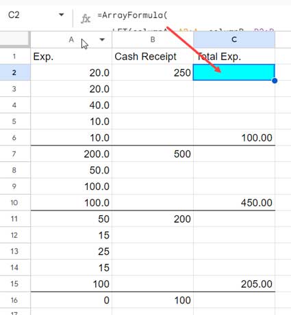
For instance, imagine you receive petty cash for daily expenses from your accountant, listed in column B. In column A, you record daily expenses against this petty cash.

With multiple cash receipts, how do you sum the expenses up to each cash receipt to track spending accurately?

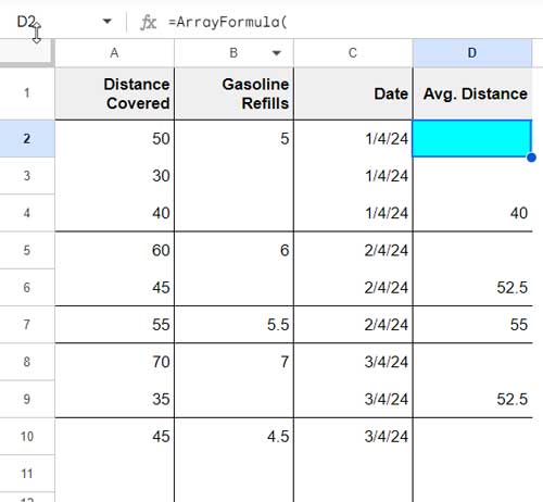
Another scenario involves tracking gasoline refills for light cranes. Each refill is listed in column B, while the daily kilometers traveled are recorded in column A. How can we determine the average distance per trip between each refill?

We can efficiently analyze column A values between non-adjacent values in column B by employing an array formula. This formula will be placed in the top row in column C and will return results in the row just above each value in column B. Please refer to the screenshot above.

Analyzing Column A Between Non-Adjacent Values in Column B: Formula and Usage Instructions

Generic Formula:

=ArrayFormula(
   LET(columnA, column_1, columnB, column_2, 
      IFNA(VLOOKUP(ROW(columnA), 
         LET(
            start, TOCOL(IF(LEN(columnB), ROW(columnB),), 1), 
            end, start-1, 
            x, CHOOSEROWS(start, SEQUENCE(COUNT(start)-1)), 
            y, CHOOSEROWS(end, SEQUENCE(COUNT(end)-1, 1, 2)), 
            HSTACK(y, 
               MAP(x, y, LAMBDA(xx, yy, function_name(
               FILTER(columnA, ISBETWEEN(ROW(columnA), xx, yy)))))
            )
         ), 2, FALSE)
      )
   )
)

In this formula, you should make three changes to analyze two columns based on values in non-adjacent cells in the second column. As per our example of petty cash and daily expenses:

1. Replace column_1 with the column that contains the data breakdown, such as daily expenses or kilometers driven. As per our example, replace this text with A2:A.
2. Replace column_2 with the column containing the non-consecutive values based on which you want to analyze column_1, such as cash receipts or gasoline/diesel refills. As per our example, replace it with B:B (this should be the entire column reference, not B2:B).
3. This is the most important part: Replace function_name with functions like SUM, AVERAGE, COUNT, MIN, or MAX. As per our example, replace it with SUM.

Examples:

Formula to calculate the average distance per trip between each refill when distances covered are in column A and gasoline refills are in column B.

=ArrayFormula(
   LET(columnA, A2:A, columnB, B:B, 
      IFNA(VLOOKUP(ROW(columnA), 
         LET(
            start, TOCOL(IF(LEN(columnB), ROW(columnB),), 1), 
            end, start-1, 
            x, CHOOSEROWS(start, SEQUENCE(COUNT(start)-1)), 
            y, CHOOSEROWS(end, SEQUENCE(COUNT(end)-1, 1, 2)), 
            HSTACK(y, 
               MAP(x, y, LAMBDA(xx, yy, AVERAGE(
               FILTER(columnA, ISBETWEEN(ROW(columnA), xx, yy)))))
            )
         ), 2, FALSE)
      )
   )
)

You should enter this formula in the second row since the expenses (column A) start at row #2. Therefore, enter it in cell D2.

Formula to sum expenses in column A based on the non-adjacent cash receipts in column B:

In the above formula, replace AVERAGE with SUM.

Formula Breakdown: Sum Column A Between Non-Adjacent Values in Column B

This section is for those interested in understanding the logic behind the formula and creating customized formulas based on this logic. I’ll explain the formula step by step and provide screenshots where necessary.

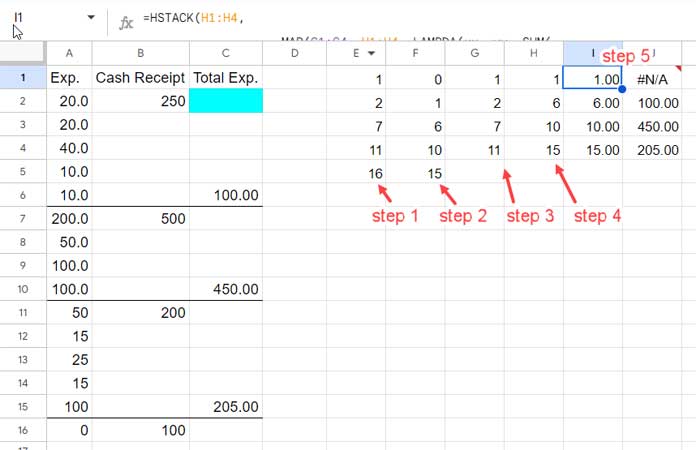
Step 1:

TOCOL(IF(LEN(columnB), ROW(columnB),), 1) – This returns the row numbers of the non-blank cells in column B. We’ve named this result “start” using the LET function.

You can test this result with:

=ArrayFormula(TOCOL(IF(LEN(B:B), ROW(B:B),), 1))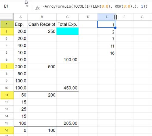

Step 2:

start-1 – This subtracts 1 from the result obtained in Step 1. We’ve named this result “end”.

You can test this with:

=ArrayFormula(TOCOL(IF(LEN(B:B), ROW(B:B),), 1)-1)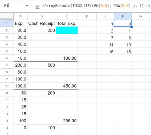

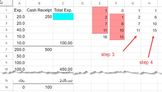
Step 3:

CHOOSEROWS(start, SEQUENCE(COUNT(start)-1)) – This removes the last value from “start”. We’ve named this result “x”.

Step 4:

CHOOSEROWS(end, SEQUENCE(COUNT(end)-1, 1, 2)) – This removes the first value from “end”. We’ve named this result “y”.

Step 5:

HSTACK(y,
MAP(x, y, LAMBDA(xx, yy, SUM(
FILTER(columnA, ISBETWEEN(ROW(columnA), xx, yy)))))
)

Here, we use the MAP function to iterate over each value in ‘x’ and ‘y’, which are part of the filter condition. The FILTER formula filters column A if its row numbers are between the values in x and y, represented by ‘xx’ and ‘yy’. The SUM function aggregates the filtered values.

The HSTACK function stacks “end” with the output to generate a lookup table.

Step 6 (Final Part):

VLOOKUP(
ROW(columnA),
…, 2, FALSE
)

The VLOOKUP formula searches the row numbers of A2:A in this table and returns the values from the second column.

That’s the logic behind the formula that dynamically analyzes column A between non-adjacent values in column B.

Resources

Here are a few related topics on analyzing a column based on non-adjacent values in another column in Google Sheets.

• How to Include Adjacent Blank Cells in Sumif Range in Google Sheets
• Group and Sum Data Separated by Blank Rows in Google Sheets
• Add Total Based on Each Change in a Column Value in Google Sheets
• AT_EACH_CHANGE Named Functions in Google Sheets