The AT_EACH_CHANGE Named Functions offer a versatile way to insert calculated summary outputs, such as totals or other aggregations, at each group change in Google Sheets. These functions simplify repetitive tasks, making them invaluable for users managing grouped data.
Let’s explore their capabilities and usage in detail.
What Are AT_EACH_CHANGE Named Functions?
The AT_EACH_CHANGE Named Functions help you insert the calculated output of summary functions at either the start or the end of each group in a dataset. These summary functions include:
- Sum
- Count
- Counta
- Max
- Min
- Average
- Product
- Standard Deviation (sample/population)
- Variance (sample/population)
Each function has a unique name, such as SUM_AT_EACH_CHANGE, AVG_AT_EACH_CHANGE, MIN_AT_EACH_CHANGE, etc., but shares the same syntax for consistency.
For instance:
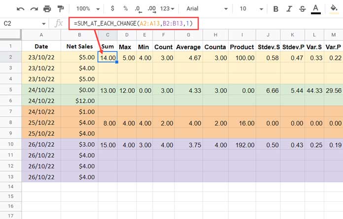
=SUM_AT_EACH_CHANGE(A2:A13, B2:B13, 1)inserts the subtotal in the first row of each group.
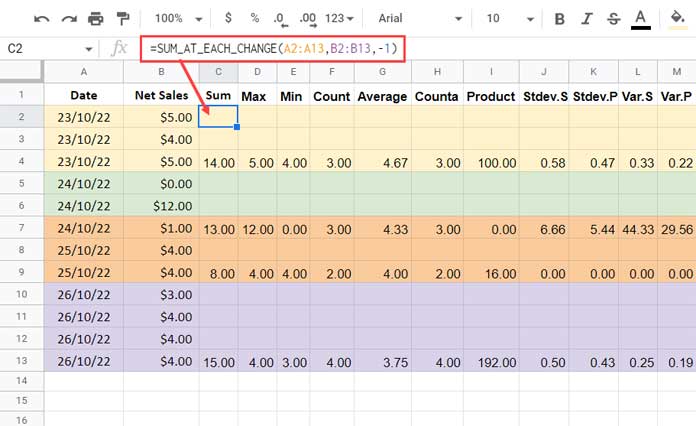
=SUM_AT_EACH_CHANGE(A2:A13, B2:B13, -1)inserts the subtotal in the last row of each group.
Syntax and Arguments
Here’s the syntax for these Named Functions:
FUNCTION_NAME(group_range, subtotal_range, mode)Arguments:
group_range: The range to test for value changes. Ensure this range is sorted.subtotal_range: The range to calculate the aggregation (Sum, Count, etc.).mode: Determines the placement of the summary values. Use1for the first row and-1for the last row of each group.
Usage Notes
- Ensure that the
group_rangedoes not contain blank cells, as they may cause#N/Aerrors. If blank cells are unavoidable, wrap the formula with IFNA to handle these errors gracefully. Note that blank rows are excluded from the aggregation. - If your
group_rangecontains 100 rows, ensure there are 99 blank rows below the formula to prevent#REFerrors. - The functions support open ranges (e.g.,
A2:A), allowing them to dynamically adjust to changes in your dataset. When using open ranges, consider wrapping the formula with IFNA for error handling.
Advantages of AT_EACH_CHANGE Named Functions
- User-Friendly: Ideal for beginners, eliminating the complexity of modifying advanced formulas.
- Time-Saving: Experts can quickly implement complex operations without repeated manual adjustments.
- Reusable: Easily import these functions into your Sheets and apply them to any dataset.
We’ve curated a growing library of custom Named Functions that you can explore and use. Visit our dedicated section here to find more.
Examples
Below are examples of common aggregations using the AT_EACH_CHANGE Named Functions. For visual reference, see Images #1 and #2.
1. Max at Each Group Change:
=MAX_AT_EACH_CHANGE(A2:A13, B2:B13, -1)2. Min at Each Group Change:
=MIN_AT_EACH_CHANGE(A2:A13, B2:B13, -1)3. Average at Each Group Change:
=AVG_AT_EACH_CHANGE(A2:A13, B2:B13, -1)How to Import and Use These Functions
Follow these steps to start using the AT_EACH_CHANGE Named Functions:
- Make a Copy: Copy the example sheet linked below.
- Open Named Functions: In your Google Sheet, go to the Data menu and select Named Functions.
- Import Functions: Click Import in the sidebar and select the desired functions from the copied example sheet.
That’s it! You’re ready to use these powerful functions.
Complete List of Functions
Below is the complete list of AT_EACH_CHANGE Named Functions you can import and use. All functions follow the same syntax.
SUM_AT_EACH_CHANGE– SumCOUNT_AT_EACH_CHANGE– CountCOUNTA_AT_EACH_CHANGE– CountaAVG_AT_EACH_CHANGE– AverageMAX_AT_EACH_CHANGE– MaxMIN_AT_EACH_CHANGE– MinPRODUCT_AT_EACH_CHANGE– ProductSTDEVS_AT_EACH_CHANGE– StdDev (sample)STDEVP_AT_EACH_CHANGE– StdDevp (population)VARS_AT_EACH_CHANGE– Var (sample)VARP_AT_EACH_CHANGE– Varp (population)
Final Thoughts
The AT_EACH_CHANGE Named Functions are a game-changer for anyone working with grouped data in Google Sheets. They’re simple, flexible, and save a significant amount of time.
Have you tried these functions? Share your feedback and let us know how they’ve helped you. Your input can inspire the development of even more powerful tools for Google Sheets users.
Thanks for visiting, and happy data processing!


Hi, cool custom function! Works well. I might suggest it would be more effective as a single function and a CHOOSE function that selects which of the 11 functions to use (same as the existing SUBTOTAL function).
Also, you might already know this, but for Google Sheet’s custom functions, you don’t have to use the outer LAMBDA wrapper as the custom function interface already does that. Just start with the BYCOL part and it is easier to enter and adapt later. 🙂
Thanks a ton for all your posts and tips.
Hi, McKay,
Thanks for your valuable feedback. I’ve taken note of it.
Hi Prashanth,
Thanks for the help.
I solved the problem using the Query function with Group and Pivot.
I put the notes of the periods in separate columns, and I used a formula from infoinspired.com to calculate the average, as you mentioned in a helper column.
Hi, Harvi,
Thanks for your feedback.
Hi Prashanth,
Thank you very much for AT_EACH_CHANGE Named Functions.
I work in a school, and I need to calculate the average of the students in several subjects over the three periods of the year.
It is like using average if set, where the criteria are the name of the student, the subject, the period, and the respective grade.
Hi, Harvi,
It might be possible. You must use a helper column to combine other criteria columns like =Arrayformula(A2:A&B2:B&C2:C) and use that in group_range.
I could help if you include an example sheet URL in your reply below.