Google Sheets IFNA function is useful to get rid off #N/A errors in formulas. Why this specific function is required when we can use IFERROR for the same purpose?
I will answer this question after introducing to you how to use the IFNA function in Google Sheets.
Syntax:
IFNA(value, value_if_na) Arguments:
value – The value to evaluate for an #N/A error.
value_if_na – The value to return if the evaluated value, the first argument, is an #N/A error.
Purpose:
The IFNA function in Google Sheets can return a specified value if the evaluated value argument is an #N/A error. That’s the one and only purpose of this logical function.
Example to IFNA Function in Google Sheets:
Here are two formulas.
The value to evaluate (first argument) in the below formula is an #N/A error. So this formula would return the specified value (value_if_na), i.e. “error”
=ifna(#N/A,"error")This formula would return 100.
=ifna(100,"error")Common Functions That Return #NA Error in Google Sheets
Vlookup, Hlookup, Match, Switch, and IFS are the main functions that return #N/A errors.
Here are a few examples.
How to Remove Vlookup #N/A Error with IFNA Function in Google Sheets
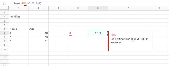
The Vlookup function (Hlookup also) would return an #N/A error if the search key is not available in the first column (first row in the Hlookup) of the lookup range.

In this Vlookup the search key is “D” which is not available in the first column in the lookup range A6:B8.
How to remove this #N/A error and return blank or a specific value in Google Sheets? You can use the Vlookup formula as below.
=ifna(vlookup(D6,A6:B8,2,0),"Not Found")If you want blank instead of the said error in Vlookup, modify the formula as given below.
=ifna(vlookup(D6,A6:B8,2,0),)#N/A Error in Match and How to Remove It
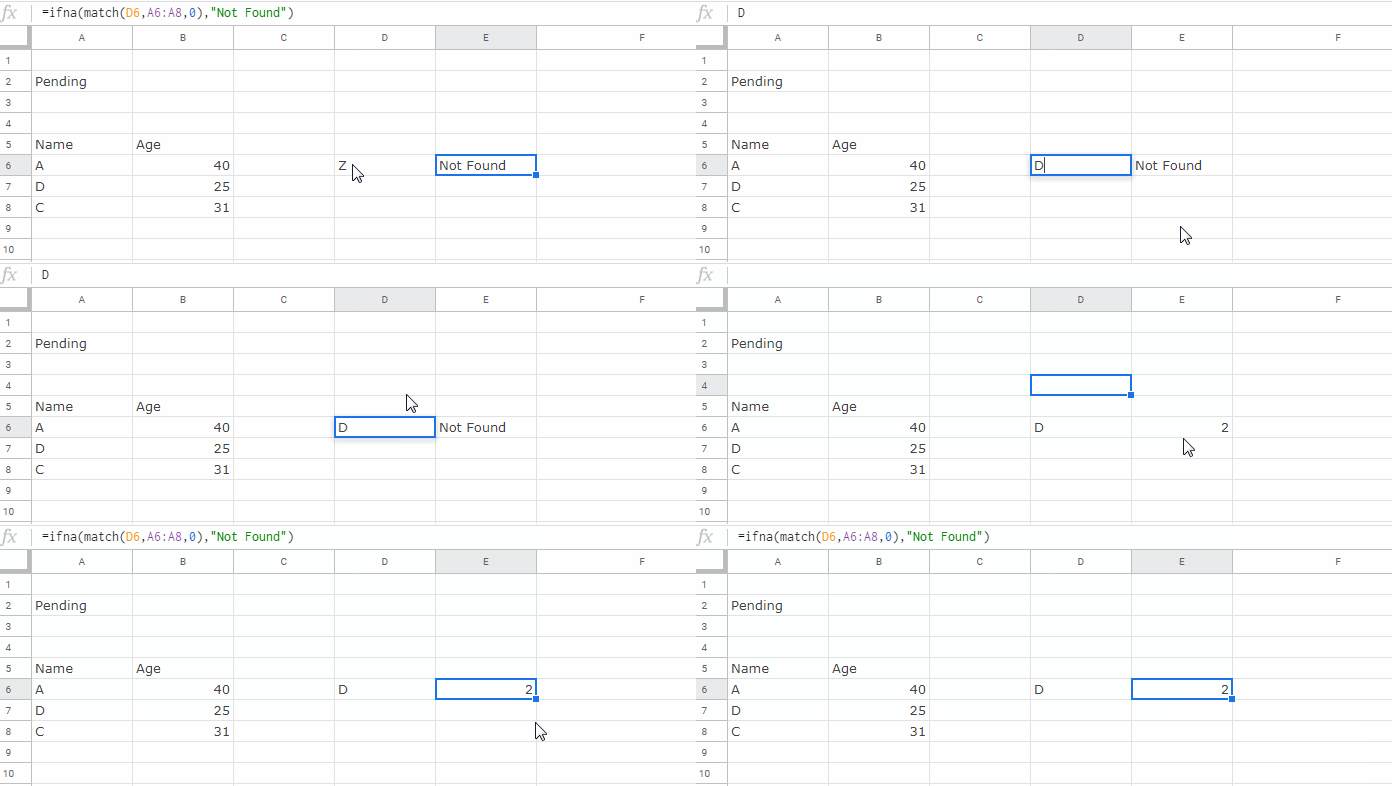
Similar in Vlookup we can use the IFNA function in Google Sheets with the Match function.
Here is one example.
=ifna(match(D6,A6:A8,0),"Not Found")
Sheets IFNA Function to Remove #N/A Error in IFS Function
IFS is another function that returns the above error. It’s not so common in use but understanding the usage may be useful.
Assume the value in cell A1 is 40.
=ifs(A1>50,"Passed")Try the above formula and see the result yourself. Here I would recommend you to use the IFS formula as below.
=ifna(ifs(A1>50,"Passed"))Another function that would return an #N/A error is SWITCH.
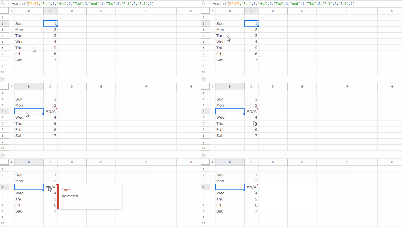
How to Remove Switch Function #N/A Error

Here you can rewrite the SWITCH formula as below.
=ifna(switch(B2:B8,"Sun",1,"Mon",2,"Tue",3,"Wed",4,"Thu",5,"Fri",6,"Sat",7))The Advantage of Using Google Sheets IFNA Function Over Iferror
In all the above examples, you can replace IFNA with IFERROR. But I won’t recommend you to use IFERROR function as an alternative to IFNA. Why?
The error value #N/A simply says the search key is not found or there is no matching key in the range. So isn’t an error exactly.
If you use IFERROR, you are eliminating your chance to audit your formula for errors!
Additional Resources:


