SUMIFS and SUMIF are infamous for producing an “argument must be a range” error when using an expression as the sum range. However, when XLOOKUP is employed as the sum range in SUMIFS, this error does not arise.
Therefore, we can use SUMIFS with XLOOKUP to conditionally sum an XLOOKUP result in Excel and Google Sheets.
In this combo, XLOOKUP looks up and returns an array using one of its advanced lookup capabilities, such as searching from last value to first value, first value to last value, approximate match, exact match, wildcard match, etc. SUMIFS then sums the values based on conditions.
This post contains a common example applicable to both Excel and Google Sheets.
An Example of SUMIFS with XLOOKUP in Excel and Google Sheets
The sample data consists of employee names in column A and their monthly salaries from January to December in columns B to M.
We will utilize XLOOKUP to search for a name in column A and retrieve their 12-month salary, then sum it across specific months using SUMIFS.
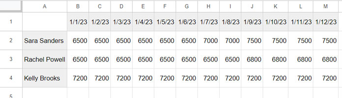
In the table above, I want to find the total salary of “Rachel Powell” in October, November, and December (4th quarter) of 2023.
Here are the step-by-step instructions:
XLOOKUP Part:
Syntax: XLOOKUP(search_key, lookup_range, result_range, [missing_value], [match_mode], [search_mode])
This is the XLOOKUP syntax in Google Sheets. You can follow the same in Excel, although the parameter names slightly vary.
In Excel, search_key will be lookup_value, lookup_range will be lookup_array, result_range will be return_array, and missing_value will be if_not_found. They refer to the same. The last two parameter names, i.e., match_mode and search_mode, are the same in XLOOKUP in Excel and Google Sheets.
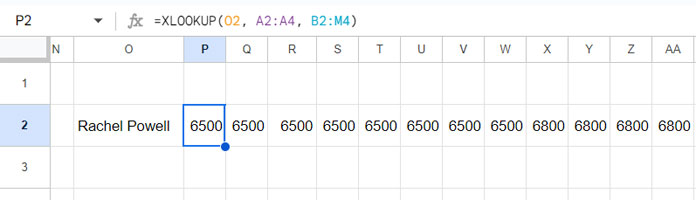
Enter the employee name (search_key) in cell O2, which is “Rachel Powell”.
Enter =XLOOKUP(O2, A2:A4, B2:M4) in cell P2 to look up the name in cell O2 in A2:A4 and return the salaries from B2:M4.
If the formula fails to expand, the formula may return a #SPILL error in Excel and a #REF error in Google Sheets. In that case, ensure that P2:AA2 doesn’t contain any values.
How to SUMIFS this XLOOKUP result? We can see that below.
SUMIFS Part:
Syntax: SUMIFS(sum_range, criteria_range1, criterion1, [criteria_range2, …], [criterion2, …])
The SUMIFS syntax is the same in both Excel and Google Sheets. Now let’s dive straight into the SUMIFS and XLOOKUP combo formula.
=SUMIFS(XLOOKUP(O2, A2:A4, B2:M4), B1:M1, ">="&DATE(2023, 10, 1), B1:M1, "<="&DATE(2023, 12, 1))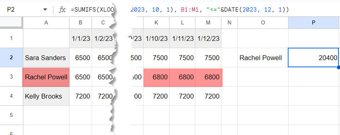
Where:
sum_range:XLOOKUP(O2, A2:A4, B2:M4)criteria_range1: B1:M1criterion1:">="&DATE(2023, 10, 1)– the date is entered according to the syntaxDATE(year, month, day)criteria_range2: B1:M1criterion2:"<="&DATE(2023, 12, 1)– the date is entered according to the syntaxDATE(year, month, day)
The SUMIFS function sums the XLOOKUP result matching the dates in the header row of the table.
This is an example of SUMIFS with XLOOKUP in Excel and Google Sheets.
What if I Have Month Names Instead of Month Start Dates?
As you can see in the sample data, B1:M1 contains the month start dates. I mean 1/1/23 represents January, and 1/12/23 represents December. So we have used dates as criteria in SUMIFS.
You may have a reason to use month texts such as January, February, … December instead in B1:M1.
In that case, you can convert those month texts to month numbers within the SUMIFS and XLOOKUP combo formula in Google Sheets and outside the formula in Excel. This is because of the dynamic array difference in both applications.
In Google Sheets:
Replace B1:M1 (appears twice) in the SUMIFS and XLOOKUP combo formula with DATE(2023, MONTH(B1:M1&1), 1). Then wrap the formula with the ARRAYFORMULA function as follows:
=ArrayFormula(SUMIFS(XLOOKUP(O2, A2:A4, B2:M4), DATE(2023, MONTH(B1:M1&1), 1), ">="&DATE(2023, 10, 1), DATE(2023, MONTH(B1:M1&1), 1), "<="&DATE(2023, 12, 1)))In Excel, enter =DATE(2023, MONTH(B1:M1&1), 1) in cell P1, provided P1:AA1 are blank. Then replace B1:M1 (twice) in the formula with P1:AA1.
Conclusion
This tutorial covered SUMIFS with XLOOKUP in Excel and Google Sheets.
If you want to explore more XLOOKUP examples in Google Sheets, including beginner tutorials, advanced lookup techniques, and real-world use cases, check out the Complete Guide to XLOOKUP in Google Sheets.


