This post describes how to use the XLOOKUP function on visible data in Google Sheets. I’ll show you how to achieve this using a LAMBDA-based LHF with the SUBTOTAL function.
We can temporarily hide unwanted or unused data in Google Sheets in 2–3 ways. The most popular options are the Filter (via Data > Create a filter) and Slicer.
I’m sure you’re familiar with those methods. There are a few others as well, such as:
- View > Group > Group rows
- Right-clicking on selected row(s) and choosing Hide row(s)
- Data > Create group by view
- Filters created via “Create a Table”
The Limitation of XLOOKUP with Hidden Rows
The XLOOKUP function has many flexible options for looking up values. But unfortunately, it does not have a built-in way to exclude hidden rows.
To XLOOKUP visible data in Google Sheets, we need to pair it with another function—SUBTOTAL.
However, the drawback is that SUBTOTAL isn’t an array formula—it doesn’t “spill” down rows automatically. To work around this, we can use a BYROW or MAP LHF (LAMBDA Helper Function).
These will allow us to expand or “spill” the SUBTOTAL results across multiple rows. I prefer the BYROW function for this purpose.
How to XLOOKUP Visible Data in Google Sheets
The XLOOKUP function offers several options to customize how a search key is matched—via match mode and search mode. I won’t go into those here since I’ve already covered them in detail in a separate tutorial.
Instead, we’ll focus on a simple example to help you understand how to use XLOOKUP with visible data in Google Sheets. If you have further questions, feel free to post them in the comments below.
Sample Data (Unfiltered)
We have a list of item codes in column A and corresponding quantities in column B. The data is currently unfiltered.
Let’s say we want to retrieve the quantity for the first item that ends with 1003. Here’s how we can do that using a wildcard match with XLOOKUP:
=XLOOKUP("*1003", A2:A, B2:B, "Not Available!", 2, 1)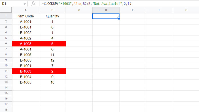
XLOOKUP Partial Match – Explained
Syntax:
XLOOKUP(search_key, lookup_range, result_range, [missing_value], [match_mode], [search_mode])search_key:"*1003"lookup_range:A2:Aresult_range:B2:Bmissing_value:"Not Available!"match_mode:2(wildcard match)search_mode:1(search top to bottom)
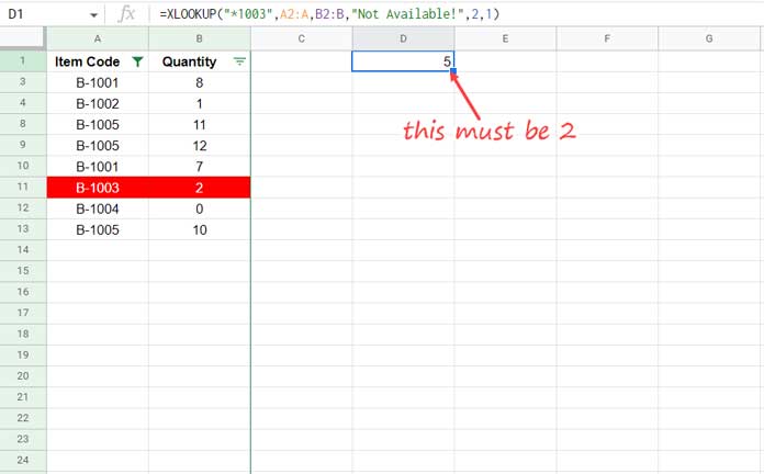
Sample Data (Filtered) – XLOOKUP in Visible Data
Now let’s apply a filter to columns A and B:
- Select the range A1:B.
- Go to Data > Create a filter.
- Click the filter icon in cell A1.
- Choose Filter by condition > Custom formula is.
- Enter the following formula:
=NOT(REGEXMATCH(A2, "(?i)^A")) - Click OK.
This hides all rows where the values in column A start with the letter “A”.”
The Problem
Here’s the issue: when you use the same XLOOKUP formula—
=XLOOKUP("*1003", A2:A, B2:B, "Not Available", 2, 1)—it still returns values from hidden rows.
The Solution: XLOOKUP Visible Data in Google Sheets
To XLOOKUP visible (filtered) data in Google Sheets, follow these steps.
Let’s use the following formula within XLOOKUP to identify which rows are visible:
BYROW(A2:A, LAMBDA(range, SUBTOTAL(103, range)))Note: SUBTOTAL(103, ...) returns 1 for visible rows and 0 for hidden rows. See the BYROW function guide for more explanation.
This returns a series of 1s and 0s depending on each row’s visibility status.
Logic Behind the Lookup
We can combine the lookup_range and visibility markers (helper formula) into one searchable array by appending a delimiter (e.g., ^) and the SUBTOTAL result. We also modify the search_key accordingly.
To avoid conflicts if your search key already includes a number like 1, it’s safer to append something like "^1" instead of just "1".
Since we’re combining arrays, we must wrap the formula in ARRAYFORMULA to ensure proper evaluation.
Here’s the final formula to XLOOKUP visible (filtered) data in Google Sheets:
=ARRAYFORMULA(XLOOKUP("*1003^1", A2:A & "^" & BYROW(A2:A, LAMBDA(range, SUBTOTAL(103, range))), B2:B, "Not Available", 2, 1))That’s it! Now your XLOOKUP will only return results from visible rows in filtered data.
Conclusion
This tutorial is part of our complete guide to XLOOKUP examples in Google Sheets. For a structured overview of basic and advanced lookup techniques, see the Complete Guide to XLOOKUP in Google Sheets.


