The purpose of the XLOOKUP function in Google Sheets is to find things in a range by row or column. For example, you can use it to search for “Mango” in one column and return its price from another column. In another example, you can search for “Ben” in one row and return his score from another row.
Previously, we used the VLOOKUP and HLOOKUP functions for these two operations. However, these functions have one limitation: they can only search down the first column (VLOOKUP) or first row (HLOOKUP) in the range. XLOOKUP does not have this limitation, so it can be used to search for values in any column or row in a range.
In XLOOKUP, we can specify whether we want an exact match, the next smaller value, the next larger value, a wildcard match, a match from the first entry to the last entry, or a match from the last entry to the first entry, etc.
For example, the following XLOOKUP formula will search for “Wheat” in column A and return the value in column C from the position found.
=XLOOKUP("Wheat",A:A,C:C,"Not Available")Prefer to watch instead of read? The full video tutorial is available at the end of this post.
XLOOKUP Function Syntax in Google Sheets
Syntax of the XLOOKUP Function in Google Sheets:
XLOOKUP(search_key, lookup_range, result_range, [missing_value], [match_mode], [search_mode])Unlike other Google Sheets functions, we must pay more attention to the arguments of the XLOOKUP function. This is because it has six arguments, which are more than most other functions.
I have moved the explanations of the arguments under two subtitles (categories) below:
- Required XLOOKUP function arguments:
search_key,lookup_range, andresult_range. - Optional XLOOKUP function arguments:
missing_value,match_mode, andsearch_mode.
With a basic understanding of these arguments, we will be able to use the XLOOKUP function effortlessly in our spreadsheets.
Required Arguments in XLOOKUP Function
The first three arguments in the XLOOKUP function are required. Below you can find their purpose and some XLOOKUP formula examples using them.
The three basic arguments are:
search_key: The value to search. For example, 156, “Apple”, Date(2022,09,20), or “ABC100”.
lookup_range: The range to consider for the search (a single column for vertical lookup and a single row for horizontal lookup).
result_range: The range to consider for the result.
Since we do not specify the optional arguments in the XLOOKUP function syntax, the formula will take their default values. That means:
- If the
search_keyis unavailable, the XLOOKUP formula will return the #N/A error value. - It will perform an exact match of the
search_key; not a match for the next smallest or largest value. - It will search from the first entry to the last entry in the
lookup_range, from top to bottom in vertical XLOOKUP, and from left to right in horizontal XLOOKUP.
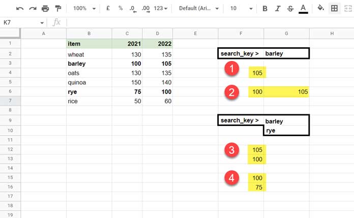
We will use the following data (please refer to Figure 1 below) for testing the XLOOKUP function with the three required arguments.
Before proceeding, if you are unfamiliar with using date, time, text, number, or datetime criteria in XLOOKUP, please check my HLOOKUP tutorial. I have a table right under the syntax part that you can refer to.
Formula Examples
1. F4 Formula:
=XLOOKUP(G2,B2:B7,D2:D7)The XLOOKUP function searches for the value “barley” (G2) in the range B2:B7 (the lookup range) and returns the value from the range D2:D7 (the result range) in the row that matches. If we consider the above data as the production of food grains in 2021 and 2022, the formula returns the production quantity of “barley” in 2022.
2. F6 Formula:
=XLOOKUP(G2,B2:B7,C2:D7)The result_range includes two columns, so the XLOOKUP formula will return values from both columns. This is an example of using a 2D array in the result range in the XLOOKUP function in Google Sheets. The result of the formula will be the production quantity of “barley” in 2021 and 2022, in a single row.
3. F12 Formula:
=ARRAYFORMULA(XLOOKUP(G9:G10,B2:B7,D2:D7))Here is an example of using multiple search keys in the XLOOKUP function in Google Sheets. The formula searches for the values “barley” and “rye” (G9:G10) in the range B2:B7 (the lookup range) and returns the values from the range D2:D7 (the result range) in the rows that match. The formula returns the production quantities of “barley” and “rye” in 2022.
When using multiple search keys in the XLOOKUP function, you must use the ARRAYFORMULA function with it. It tells Google Sheets to return an array of values, which is what you need when using multiple search keys in the XLOOKUP function.
4. F15 Formula:
=ARRAYFORMULA(XLOOKUP(G9:G10,B2:B7,C2:D7))Here, the XLOOKUP result_range includes two columns. However, since there is more than one search_key, the formula will only return values from the first column. This is because the XLOOKUP function is not capable of returning 2D arrays.
We can solve the issue of XLOOKUP not returning a 2D array by using a workaround that keeps all XLOOKUP flavors. This workaround involves using the CHOOSEROWS function with the XMATCH function. You can find a tutorial on how to do this here: CHOOSEROWS Function in Google Sheets.
Please understand the above thoroughly before proceeding to the optional arguments below.
Optional Arguments in XLOOKUP Function
The three optional arguments for the XLOOKUP function are:
missing_value: The value to return if no match of thesearch_keyis found.match_mode: The type of match to perform in thelookup_range.search_mode: The manner in which to search through thelookup_range.
Here is how to use them in XLOOKUP formulas:
Missing Value and Examples
Missing_value is an optional argument in the XLOOKUP function in Google Sheets. If this argument is omitted, the function will return #N/A by default if no match is found.
The following XLOOKUP formula will return “Seems there is a typo!” if the search_key is not found in the range B2:B7.
=xlookup(G2,B2:B7,D2:D7,"Seems there is a typo!")I have three search keys and one of them is not matching. What about the missing_value in this scenario?
Please see the below image (figure 2).

Match Modes in XLOOKUP Function in Google Sheets
The match_mode in the XLOOKUP function determines how to find a match for the search_key, which is the value you are looking for.
- 0: Exact match (default).
- 1: Exact match or the next value that is bigger than the
search_key. - -1: Exact match or the next value that is lower than the
search_key. - 2: Wildcard Match.
Formula Examples
In the following examples, we have the interview dates in column B and the names of candidates in column C.
Let’s use the XLOOKUP function to find the candidate on a particular date. If no candidate is available on that date, return the candidate on the previous or next date.
Formula:
=XLOOKUP(D3,B3:B7,C3:C7,"No Appointment",1)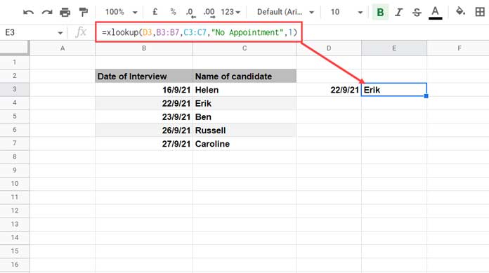
22/09/2021 (cell D3) is the date to match in column B. As you can see, it is available in column B. Therefore, regardless of the match_mode used, whether it is 0 (exact), 1 (next largest), -1 (next smallest), or 2 (wildcard), the formula will return the name “Erik”.
Change the search_key to 24/09/2021. The following exact match formula will return “No Appointment.”
=XLOOKUP(D3,B3:B7,C3:C7,"No Appointment",0)If you change the match_mode parameter of the XLOOKUP function to 1, the output will be “Russel”, and -1 will make it return “Ben.”
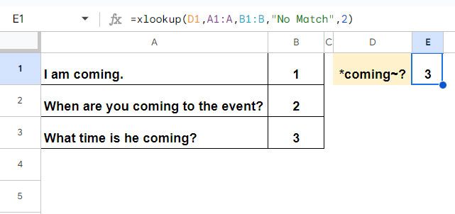
How does the wildcard match work in the XLOOKUP function in Google Sheets?
The XLOOKUP function supports three wildcard characters: an asterisk (*), a question mark (?), and a tilde (~).
| Wildcard Symbol | Description | Example |
| * (asterisk) | Represents zero or more characters. | "A*ca" matches Africa, America, or Antarctica. |
| ? (question mark) | Represents a single character. | "S?ng" matches Sing, Sung, or Sang. |
| ~ (tilde) followed by ?, *, or ~ | Identifies a wildcard character. | "coming~?" matches “coming?” |
Many people mistakenly believe that XLOOKUP supports only two wildcard characters: asterisk and question mark. Here is how to use the tilde in the XLOOKUP function in Google Sheets.
Search Modes in XLOOKUP Function in Google Sheets
The search_mode argument in the XLOOKUP function determines how to search through the lookup_range, which is the range of cells where the XLOOKUP function looks for the search_key.
Here are the 4 search modes.
- 1: Search from the first entry to the last entry (default).
- -1: Search from the last entry to the first entry.
- 2: Binary search (
lookup_rangemust be sorted in ascending order). - -2: Binary search (
lookup_rangemust be sorted in descending order).
Formula Examples
Among the four search modes, 1 and -1 are most useful when you have multiple occurrences of search keys in the lookup range.
The binary search modes 2 and -2 in the XLOOKUP function are the most confusing part. You can understand it with the help of the table below.
Note:- First, sort the data in ascending (A-Z) or descending order (Z-A). Accordingly, use search_modes 2 or -2.
| Match Mode | Search Mode | Return Position w.r.t. Duplicate |
| 0 (Exact Match) | 2 (Sorted Asc.) | First Match |
| 0 (Exact Match) | -2 (Sorted Desc.) | Last Match |
| 1 or -1 (next value > or <) | 2 (Sorted Asc.) | Closest to the insertion point |
| 1 or -1 (next value > or <) | -2 (Sorted Desc.) | Closest to the insertion point |
Let’s try to understand what “closest to the insertion point” means in the XLOOKUP function in Google Sheets.
Table: A1:B4 (Ascending [A-Z] Order)
23/9/21 | Ben
23/9/21 | Russell
26/9/21 | Andrew
26/9/21 | Charles
If the search key is 24/09/2021 in binary search mode 2, the closest date to the insertion point will be 23/09/2021 when the match mode is -1 (next smallest), or 26/09/2021 when the match mode is 1 (next largest).
Example 1:
=XLOOKUP(DATE(2021,9,24),A1:A4,B1:B4,"Not Available",-1,2)Result: “Russel”
Example 2:
=XLOOKUP(DATE(2021,9,24),A1:A4,B1:B4,"Not Available",1,2)Result: “Andrew”
Table: A1:B4 (Descending [Z-A] Order)
26/9/21 | Charles
26/9/21 | Andrew
23/9/21 | Russel
23/9/21 | Ben
Please see the bolded dates for the closest match to the search key 24/09/2021. The binary search mode is -2.
Horizontal XLOOKUP in Google Sheets
The XLOOKUP function in Google Sheets works equally well with horizontal and vertical lookup and result ranges. Here is an example that summarizes my previous explanations, but uses horizontal data.
Assume that the first row of a table contains the timescale of a project schedule. In the rows below, I have manpower allocations. Let’s see how to retrieve the manpower allocated on a particular date.
The search key is 15/07/2023 in cell A10. We will look up this date in B2:E2 and return the manpower allocated for “task 3” from B5:E5. If the search key is not available, we will retrieve the figure from the next largest date.
Since we have a sorted lookup range, we can use either binary search mode 2 or search mode 1. Of course, the match mode is 1, since we want to perform an exact or next largest date match.
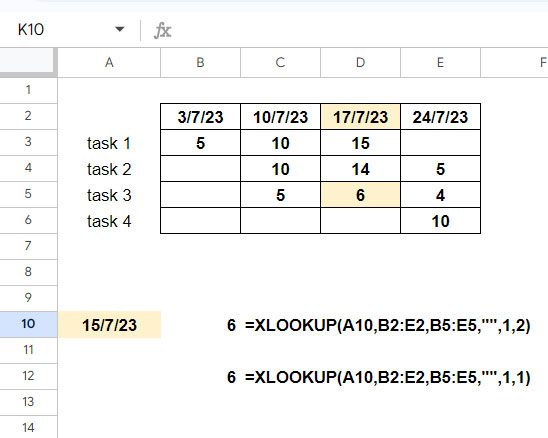
Horizontal XLOOKUP Formulas:
1: =XLOOKUP(A10,B2:E2,B5:E5,"",1,2)
2: =XLOOKUP(A10,B2:E2,B5:E5,"",1,1)
XLOOKUP in Google Sheets – Video Tutorial
Conclusion
This guide focuses on a specific use case of XLOOKUP. For a broader collection of XLOOKUP examples in Google Sheets, including advanced lookup techniques and real-world scenarios, see the Complete Guide to XLOOKUP in Google Sheets.
You can also use the FILTER function or QUERY function to filter rows or columns matching one or more lookup values.


