The XMATCH function is part of the recently launched function bundle in Google Sheets, which also includes XLOOKUP, LAMBDA, and LAMBDA Helper Functions (LHF). Another exciting feature introduced alongside this bundle is Named Functions.
You can find my posts about the other functions in this bundle in my Google Sheets Function Guide.
In this tutorial, you will learn how to use the XMATCH function through several examples.
Purpose of the XMATCH Function in Google Sheets
The XMATCH function searches for an item (referred to as search_key) and returns its relative position within a single row or column range (lookup_range). This function has various search and match modes that differentiate it from the traditional MATCH function.
Syntax and Arguments
Syntax:
XMATCH(search_key, lookup_range, [match_mode], [search_mode])Arguments:
The XMATCH function contains four arguments, with the last two being optional:
- search_key: The value (item) you want to search for.
- lookup_range: A single row or column where the search will occur.
- match_mode (optional, default is 0): Determines how the function finds a match. The options are as follows:
| MATCH MODE | DESCRIPTION |
| 0 | Exact Match |
| 1 | Exact Match or the Next Largest Value |
| -1 | Exact Match or the Next Smallest Value |
| 2 | Wildcard Match |
It’s important to note that when comparing modes 1 and -1 with those in the MATCH function, the latter requires a sorted lookup_range for approximate matches, while XMATCH does not.
- search_mode (optional, default is 1): Determines the search direction through the lookup_range. The options are as follows:
| SEARCH MODE | DESCRIPTION |
| 1 | First Entry to Last |
| -1 | Last Entry to First |
| 2 | Binary Search (lookup range must be sorted in ascending order) |
| -2 | Binary Search (lookup range must be sorted in descending order) |
How to Use the XMATCH Function in Google Sheets – Examples
Let’s explore how to match a date in a column of dates to find its relative position. For demonstration purposes, we will assume column A contains unsorted dates and column B contains corresponding names from a sample hotel room booking data set.
Exact Match and Search From First Entry to Last
Formula 1 (Exact Match):
=XMATCH(D3, A3:A12, 0, 1)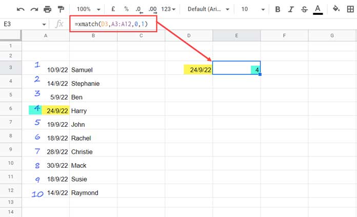
Note: You can also simplify the formula to =XMATCH(D3, A3:A12) because the last two arguments are set to their default values (0 for match_mode and 1 for search_mode).
This formula searches for the date 24/09/2022 in the range A3:A12 and returns the relative position of the matching date, which is 4.
We can combine this with the INDEX function to return the name of the person who booked the room:
=INDEX(B3:B12, XMATCH(D3, A3:A12), 1)Approximate Match and Search From First Entry to Last
What if the search_key in cell D3 is 17/09/2022? Since this date does not exist in the list, the formula would return #N/A. However, if we use match_mode 1, it will find the next largest value, 18/09/2022.
Formula 2 (Next Largest):
=XMATCH(D3, A3:A12, 1)The relative position of the date 18/09/2022 in the list is 6.
To return the name of the person who booked the room on that date, we can use:
=INDEX(B3:B12, XMATCH(D3, A3:A12, 1), 1)Next Smallest:
To find the next smallest date, we can use:
=XMATCH(D3, A3:A12, -1)This will return 2 as the relative position of the date 14/09/2022.
Search From Last Entry to First in the XMATCH Function
So far, all the examples have used the default search mode (1), which searches from the first entry to the last. Let’s explore how the results change when we search from the last entry to the first (-1).
Exact Match:
=XMATCH(D3, A3:A12, 0, -1)For the exact match with the date 24/09/2022, this formula will still return 4 since there are no duplicates.
Next Largest:
=XMATCH(D3, A3:A12, 1, -1)Here, the next largest date to 17/09/2022 is 18/09/2022, which has a relative position of 9 when searching from the bottom.
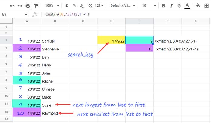
Next Smallest:
=XMATCH(D3, A3:A12, -1, -1)The next smallest date, 14/09/2022, has a relative position of 10 when searching from the bottom.
Note: The difference between searching from first to last and last to first is significant when there are duplicate entries in the lookup_range.
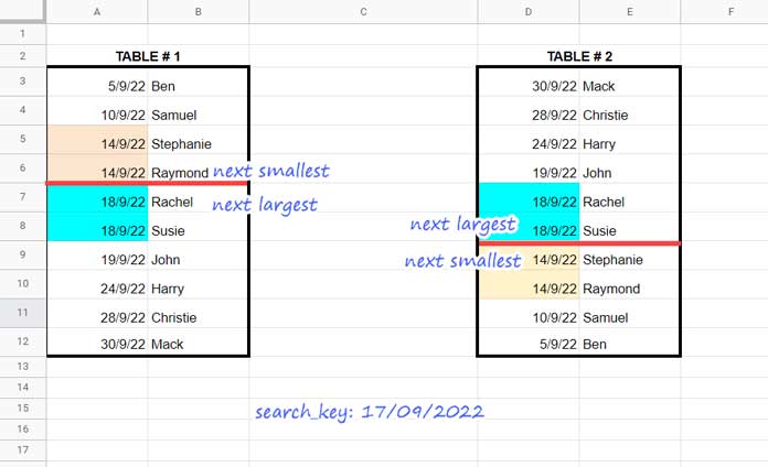
Binary Search Modes (2 and -2)
For faster lookups, you can sort the lookup_range in ascending or descending order. The binary search modes support exact matches, the next smallest, and the next largest matches.
Example for Binary Search in Ascending Order:
=XMATCH("apple", {"apple"; "apple"; "orange"; "orange"}, 0, 2)This will return 1.
Example for Binary Search in Descending Order:
=XMATCH("apple", {"orange"; "orange"; "apple"; "apple"}, 0, -2)This will return 4.
Next Largest and Next Smallest Matches in Binary Search Mode
Using the date 17/09/2022:
For Ascending Order:
Next Largest:
=XMATCH(DATE(2022, 9, 17), A3:A12, 1, 2)Output: 5
Next Smallest:
=XMATCH(DATE(2022, 9, 17), A3:A12, -1, 2)Output: 4
For Descending Order:
Next Largest:
=XMATCH(DATE(2022, 9, 17), D3:D12, 1, -2)Output: 6
Next Smallest:
=XMATCH(DATE(2022, 9, 17), D3:D12, -1, -2)Output: 7
How to Use Wildcards in the XMATCH Function
The XMATCH function also supports wildcards. For instance, if you want to find the last total amount in column C, regardless of whether the label in the corresponding row in column B is “Total,” “Sub Total,” or “Grand Total,” you can use the following combination:
=INDEX(C:C, XMATCH("*Total*", B:B, 2, -1))Wildcard Table:
| Wildcard Symbol | Description | Example |
| * | Represents zero or more characters | “*Total*” finds Total, Sub Total, or Grand Total. |
| ? | Represents a single character | “S?ng” finds Sing, Sung, or Sang. |
| ~ | Identifies a wildcard character | “coming~?” finds “coming?” |
Conclusion
That’s it for the XMATCH function! Thank you for reading, and I hope you found this guide helpful. Enjoy exploring the features of Google Sheets!


