XMATCH Multiple Columns in Google Sheets

This tutorial will teach you how to use the XMATCH function to search for a value across multiple columns in Google Sheets. You’ll learn step-by-step how to create and modify the formula to suit your needs.

Introduction to XMATCH

The primary purpose of match functions, such as MATCH or XMATCH, in Google Sheets is to find the position of an item within a column or row. They return a number relative to the rows (for vertical searches) or columns (for horizontal searches) in the array, not the entire spreadsheet. This number can then be used as a reference or combined with other functions like INDEX, FILTER, QUERY, and more for additional tasks.

The XMATCH function is designed to search within a one-dimensional array. It requires at least two arguments:

search_key: The value you are searching for.
lookup_range: The range of cells to search (must be one-dimensional).

Here’s the syntax for the XMATCH function in Google Sheets:

XMATCH(search_key, lookup_range, [match_mode], [search_mode])

The Challenge

Using XMATCH across multiple columns typically involves dragging the formula horizontally to reference different columns. However, this approach isn’t practical when you want to integrate XMATCH with other functions, such as INDEX or FILTER.

So, how can we expand the XMATCH lookup range to include all columns in a table without dragging the formula?

We can solve this using the MAP function (a type of LAMBDA function) in combination with other functions.

XMATCH Across Multiple Columns Without Dragging

Scenario:

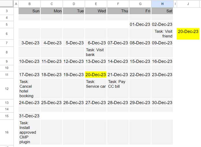
Assume you have a calendar view template in Google Sheets with data in the range B3:H16. The date you want to search for is in cell J6.

Calendar View and Date Matching in Google Sheets

Standard Approach (Dragging Formula):

To search for the date using XMATCH, you might use this formula in cell K6 and drag it across:

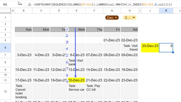
=XMATCH($J$6, B3:B16)

If the date is found in the fourth column, the formula will return 9. This is because:

$J$6 is an absolute reference (fixed).
B3:B16 is a relative reference, which adjusts as you drag the formula across columns.

Limitations:

Dragging formulas can lead to inefficiencies, especially when working with larger datasets or when integrating with other functions.

Advanced Solution Using MAP

To eliminate the need to drag formulas, we can use the MAP function to apply XMATCH to all columns in the range simultaneously. Here’s the final formula:

=SORTN(
   MAP(
      SEQUENCE(COLUMNS(B3:H16)), 
      LAMBDA(col, XMATCH(J6, INDEX(B3:H16, 0, col)))
   )
)

Example of using XMATCH to search for a value in multiple columns.

Important: If you want to retrieve matching results from all columns, remove the SORTN() wrapper. Without it, the results will be an array like:

{#N/A; #N/A; #N/A; 9; #N/A; #N/A; #N/A}

This output indicates that the match is found in the fourth column of the range.

Formula Breakdown

1. Base Formula

=XMATCH($J$6, INDEX(B3:H16, 0, 1))

INDEX(B3:H16, 0, 1) extracts the first column of the range.
This base formula searches for the value in cell J6 within that column.

2. Creating a Virtual Array:

To search across all columns, create a virtual array representing the column numbers using SEQUENCE and COLUMNS:

=SEQUENCE(COLUMNS(B3:H16))

This array represents each column number in the range B3:H16.

3. Using MAP

The MAP function applies the XMATCH formula to each column in the array:

col iterates through the column numbers.
INDEX(B3:H16, 0, col) extracts each column for XMATCH to search.

Returning Values Based on Matches

Return Value from a Matching Row

To return a value from the matching row in another column, combine XMATCH with INDEX:

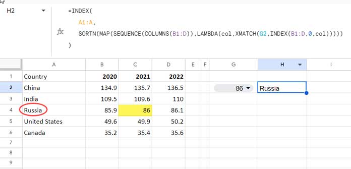
=INDEX(
   A1:A,
   SORTN(
      MAP(
         SEQUENCE(COLUMNS(B1:D)), 
         LAMBDA(col, XMATCH(G2, INDEX(B1:D, 0, col)))
      )
   )
)

A1:A: The reference column to return values from (e.g., country names).
SORTN: Returns the first non-#N/A match.

XMATCH multiple columns and return value from a chosen column

Return Value from a Matching Column

To return the header or values related to the matching column, use LET to simplify the formula:

1. Return Header:

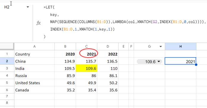
=LET(
   key,
   xmatch_formula,
   INDEX(B1:D, 1, XMATCH(1, key, 1))
)

Explanation:

key: This represents the array returned by the xmatch_formula. Ensure the SORTN wrapper is removed from the formula to retain all matches, including #N/A values.
INDEX(B1:D, 1, XMATCH(1, key, 0)): This retrieves the header (first row) from the matching column, as the row argument is set to 1.

XMATCH multiple columns and return value from a chosen row

2. Return Value Below Match:

=LET(
   key,
   xmatch_formula,
   INDEX(B1:D, SORTN(key)+1, XMATCH(1, key, 1))
)

3. Return Value Above Match:

Replace +1 with -1 in the formula above.

Conclusion

You can adapt the XMATCH function in Google Sheets to efficiently search across multiple columns using MAP. By eliminating the need for dragging formulas and incorporating advanced techniques, you can streamline your workflows and integrate XMATCH seamlessly with other functions.

Related Topics: