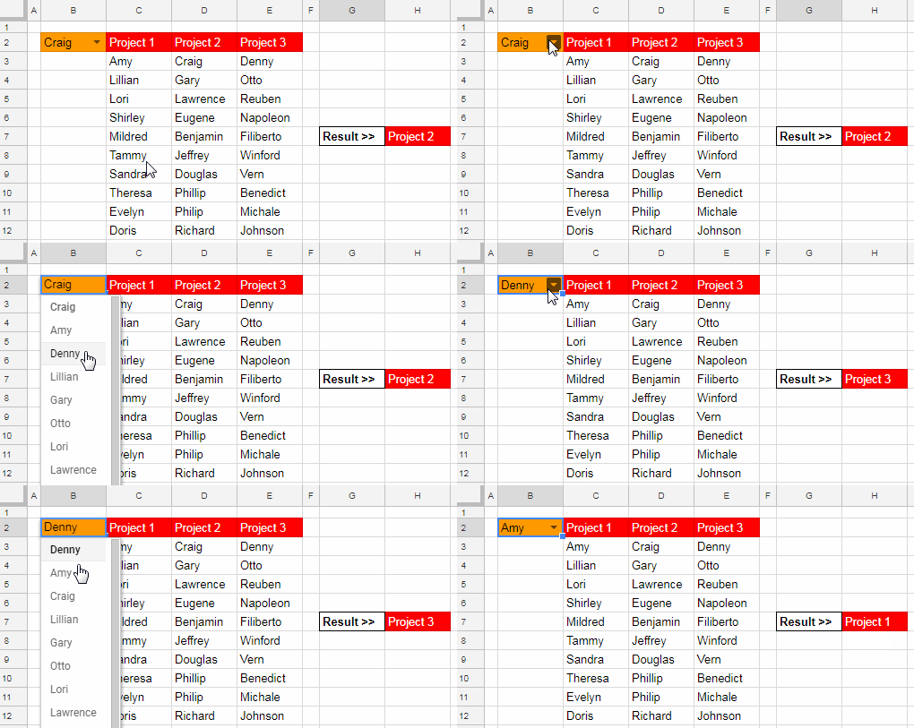
To search across columns and return the header, the best formula in Google Sheets would be a Match formula.
But when the number of columns is large, then the Match won’t help. Here comes the importance of this tutorial.
I am using a dynamic Query for searching a keyword across multiple columns, or you can say the cells in a data range and return the corresponding column header.
Searching across columns for a search key may be a rare scenario, but handy at times.
Example to Search Across Columns and Return the Header
Below, the search key is in cell B2, and the search columns are C, D, and E.

Since there are only three columns to search, you can use the Match formula.
=ifs(isna(match(B2,C3:C12,0))=FALSE,C2,isna(match(B2,D3:D12,0))=FALSE,D2,isna(match(B2,E3:E12,0))=FALSE,E2)Note:- To learn the functions in use individually, please check my Sheets functions guide.
The above formula searches the keyword provided in cell B2 in multiple columns (C, D, and E) and returns the header of the found column.
In a real-life scenario, you can say the formula searches employee names in multiple columns and return the project assigned to him.
This formula won’t be viable if the number of columns is large.
For example, in a 10-column data range, you may find coding it a tedious job.
Dynamic Formula to Search Across Multiple Columns and Return the Header
Update:- It’s an old-school approach. I’ve added a new Lambda solution at the end of this tutorial.
I have a dynamic formula to search a value in multiple columns in Google Sheets and return the field label, or you can say the header.
You May Like:- Column Heading | Column Label | Column Name | Field | Field Label in Google Sheets.
If you have 1-3 columns, please use the above Match formula.
If the number of columns is more than 3, then use the Query below. Please note that it will work for any number of columns.
=Query(transpose(query({C2:E},"Select * where "&join(" or ",ArrayFormula("Col"&column(C2:E2)-column(C2)+1&" ='"&B2&"'")),1)),"Select Col1 where Col2='"&B2&"'",0)This formula is for searching the above same column range C2:E (three columns).
Change the C2:E (it comes twice in the formula) reference to increase or decrease the search columns.
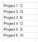
For example, if the range is C2:H (6 columns), change the formula as below.
=Query(transpose(query({C2:H},"Select * where "&join(" or ",ArrayFormula("Col"&column(C2:H2)-column(C2)+1&" ='"&B2&"'")),1)),"Select Col1 where Col2='"&B2&"'",0)So use the above dynamic formula to search across columns and return the header in Google Sheets.
Formula Explanation (Search Multiple Columns)
Let me take you through every step involved in developing this Query formula.

The above is a combination of two Query formulas.
Here is the inner Query, which returns the row that contains the search key.
=query({C2:H},"Select * where "&join(" or ",ArrayFormula("Col"&column(C2:H2)-column(C2)+1&" ='"&B2&"'")),1)How does it be able to return the row number?
I’ll come to that later (See dynamic OR columns below).
Here is the output.

In the master formula, as you can see, the inner Query is wrapped by the Transpose. That makes the above output vertical.

In the outer Query, this two-column data is the range.
It returns the column 1 value (header) if the column 2 value is the search key.
Dynamic OR Columns in Query
The inner Query used in the above formula is equal to using this.
=query({C2:H},"Select * where Col1='"&B2&"' or Col2='"&B2&"' or Col3='"&B2&"' or Col4='"&B2&"' or Col5='"&B2&"' or Col6='"&B2&"'",1) In this Query, the Where clause contains multiple OR conditions.
Similar: How to Use Multiple OR in Google Sheets Query.
Col1='"&B2&"' or Col2='"&B2&"' or Col3='"&B2&"' or Col4='"&B2&"' or Col5='"&B2&"' or Col6='"&B2&"'"The Query checks every column for the search key in cell B2.
It’s not advisable to use the multiple OR as above in Query.
If so, there is no point in using the Query instead of the provided Match formula to search across columns and return the header in Google Sheets.
The below formula automates the multiple OR in Query.
&join(" or ",ArrayFormula("Col"&column(C2:H2)-column(C2)+1&" ='"&B2&"'"))There is a sheer benefit of using this method, that it can include a large number of columns.
To use this in a different range, change the below cell references:
C2:H2 – range
C2 – the first cell address in the data range
B2 – the cell contains the search key (criteria)
If you want to search across multiple columns for a number, then the criteria should be used as below.
"&B2&" instead of '"&B2&"'Lambda Solution
This one will also work for several columns.
Further, if a name repeats in more than one column, it will return the header of both columns.
=textjoin(",",true,BYCOL(C2:E11,LAMBDA(c,IFNA(IF(MATCH(B2,c,0),INDEX(c,1),""),""))))Since it equally works in Excel, I’m directing you to my related tutorial here – Search a Value and Return Its Header in Excel 365.
To search multiple columns and extract the header, use the Match formula in Google Sheets only if your data contains 2-3 columns. Else go for Query or Lambda.


Thank you very much for this solution! Yes, it works, even with absolute references in the part [column($C2:$H2)-column($C$2)], if you want to drag e.g.
='"&B2&"'")to B10. Very helpful.Hello Prashanth,
I have the following test Google Sheet. My goal is to take the data from A1:O10 and list it as laid out in cells A14:F29, with the query formula being in cell A15. Is this even possible? The sheet link is provided below.
[URL]
Thanks,
Jack
Hi Jack,
You need to unstack the data. Please review the formulas entered in your sheet.
I hope that helps.
Thanks Prashanth. It is very helpful. I will go read up on unstacking data.
This is very helpful – thank you! Is it possible to make the
'"&B2&"'in the inner query a range? Or dynamic? Such as'"&B2:B&"'Hi, Jason,
Nope! But there are better options now in Google Sheets to achieve your desired goal.
Please try this.
=map(B2:B10,lambda(r,textjoin(", ",true,filter(index(split(flatten(C3:E&"|"&C2:E2),"|"),0,2),
index(split(flatten(C3:E&"|"&C2:E2),"|"),0,1)=r))))
Thank you very much!