You can join multiple conditions using the OR logical operator in QUERY to match either of the conditions. However, using OR is not ideal when dealing with many conditions, as it requires multiple OR statements. The easiest way to apply multiple OR conditions in Google Sheets QUERY is by using the MATCHES (preg) regular expression match instead of the OR logical operator.
In this tutorial, I will cover both approaches. You can use OR when there are only two or three conditions. However, if you have more conditions or need to use a list, I recommend using MATCHES.
This tutorial is part of the WHERE Clause in Google Sheets QUERY: Logical Conditions Explained hub, which covers all logical operators, comparisons, and condition-building patterns used in QUERY statements.
Applying Multiple OR Conditions in QUERY Using OR Logical Operator
Below is a sample dataset with flight timings from Dubai to various destinations. Columns A to D contain the destination, departure time, arrival time, and duration.
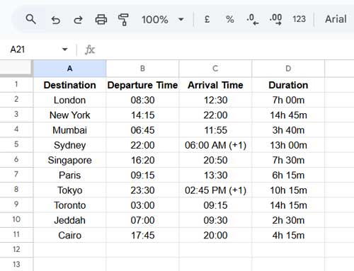
Although this is a sample dataset, please note one important detail: The departure and arrival times are in local time zones. Flight durations account for time zone differences, but this does not affect how we apply multiple OR conditions in Google Sheets QUERY.
Example 1: Hardcoded OR Conditions
Assume you want to filter destinations Singapore, London, and Mumbai:
=QUERY(A1:D, "select * where A='London' or A='Singapore' or A='Mumbai'", 1)This formula applies multiple OR conditions using the OR logical operator in the QUERY function.
Example 2: Using Cell References for OR Conditions
If the destinations to filter are in F1, F2, and F3, use the following formula:
=QUERY(A1:D, "select * where A='"&F1&"' or A='"&F2&"' or A='"&F3&"'", 1)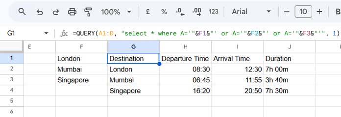
If you are unfamiliar with using different literals in QUERY, check out: Literals in Google Sheets QUERY – How to Use Them.
Applying Multiple OR Conditions in QUERY Using MATCHES
Now, let’s see how MATCHES can replace multiple OR logical operators in the QUERY function.
Example 3: Using MATCHES with Hardcoded Values
To replace the first formula above where the city names are hardcoded, use:
=QUERY(A1:D, "select * where A matches 'London|Singapore|Mumbai'", 1)This approach is simpler because you only need to separate each condition with a pipe (|).
Example 4: Using MATCHES with a Cell Range
If the criteria are listed in F1:F3, you can use:
=QUERY(A1:D, "select * where A matches '"&TEXTJOIN("|", TRUE, F1:F3)&"'", 1)Here, TEXTJOIN is used to combine the conditions with a pipe:
TEXTJOIN("|", TRUE, F1:F3)We specify it as a string literal by adding "'& on the left and &'" on the right.
Benefits of Replacing OR Logical Operators with MATCHES
Using MATCHES instead of OR logical operators has several advantages.
When hardcoding conditions, MATCHES makes the formula cleaner and easier to read.
When using a cell range for criteria, applying multiple OR conditions with the OR logical operator can become cumbersome. Instead of manually specifying each condition, you can refer to the range dynamically using TEXTJOIN. Additionally, you can make the range open-ended (e.g., F1:F) instead of specifying a fixed range like F1:F3.
Additional Tips
All the above formulas are case-sensitive. To make them case-insensitive, convert the column to lowercase using the LOWER function and ensure the criteria are also in lowercase. Here’s an example:
=QUERY(A1:D, "select * where lower(A) matches 'london|singapore|mumbai'", 1)


