Advanced substring comparison is possible with the Matches regular expression match in Google Sheets Query. Here is how to do this:
Once you have learned the basics of the Query function, you should start exploring advanced Query language features in Google Sheets.
In this tutorial, I have presented several formula examples that you may find very useful for mastering the Matches regular expression match in Google Sheets Query.
This post elaborates on how to match texts in a column with the Regex regular expression match.
This regex-based approach is covered within the broader String Matching in Google Sheets QUERY guide.
The Matches is all about Regular Expression Match in Query Function
Please note that, unlike the match in the REGEXMATCH function, the Matches regular expression match in the WHERE clause in the Query language requires the entire string to match the given regular expression. It follows a (preg) regular expression match using Perl-compatible regular Expressions (PCRE) syntax.
Let me explain this with an example. Consider the following REGEXMATCH formula and the subsequent Query:
=REGEXMATCH(A1, "Info Inspired")This REGEXMATCH formula would return TRUE if cell A1 contains the text “Info Inspired,” “Info Inspired Blog,” “New Info Inspired,” etc. It’s a global, case-sensitive match.
But the following Query formula with Matches regular expression in the WHERE Clause only filters the rows in column A that exactly match the text “Info Inspired,” and it is also case-sensitive:
=QUERY(A1:A, "SELECT A WHERE A MATCHES 'Info Inspired' ")If you want a partial match similar to the REGEXMATCH formula above, you should wrap the regular expression with .*.
=QUERY(A1:A, "SELECT A WHERE A MATCHES '.*Info Inspired.*' ")I hope this makes sense.
Matches Regular Expression Match in Query: Formula Examples
Here are some formula examples that can help you become more familiar with the Matches regular expression match in Google Sheets Query.
Query Formula to Match Either of the Texts (This or That) in Sheets
In this example, the Matches regular expression replaces the OR logical operator in the Query.
=QUERY(A1:B, "SELECT * WHERE B MATCHES 'India|Russia' ")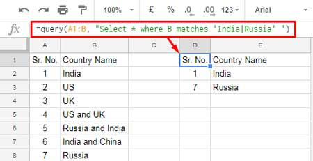
This Query formula filters the rows matching the text “India” or “Russia.”
The formula using the logical operator OR within the Query would be as follows:
=QUERY(A1:B, "SELECT * WHERE B = 'India' OR B = 'Russia'")You may also be interested in: How to Use AND, OR, and NOT in Google Sheets Query.
It’s advisable to stick with the regex approach to replace the OR logical operator if the match texts (conditions/criteria) are more than two. This way, we can keep the formula cleaner.
Query Formula to Match a Substring Anywhere in a Text String
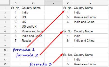
This example includes three Query formulas utilizing three different regex expressions.
First, review each formula individually, and then examine the sample sheet screenshot for the results.
The Query formulas are located in cells D1, D6, and D11.
D1:
=QUERY(A1:B, "SELECT * WHERE B MATCHES '.*India.*' ")D6:
=QUERY(A1:B, "SELECT * WHERE B MATCHES 'India.*' ")D11:
=QUERY(A1:B, "SELECT * WHERE B MATCHES '.*India' ")Take a look at the results.
We are exploring examples of the Matches regular expression match in Google Sheets Query. Let’s explore a few more formulas.
Regular Expression to Match a Text String Containing Numbers in Query
Use the formula below when you want to filter alphanumeric characters using Google Sheets Query.
Quite handy for filtering passwords in a column containing alphanumeric characters.
=QUERY(A1:B, "SELECT * WHERE B MATCHES '.*(\d).*' ")Query to Match Content Between Question Marks or Open/Close Brackets
=QUERY(A1:B, "SELECT * WHERE B MATCHES '.*\?([A-Za-z]+)\?.*'")In this formula, you can replace the question mark with open/close brackets to match the contents within brackets in a text.
Example:
=QUERY(A1:B, "SELECT * WHERE B MATCHES '.*\(([A-Za-z]+)\).*'")It matches texts like “info inspired (tech) blog,” which contains text inside the open/close brackets.
For a more specific match:
=QUERY(A1:B, "SELECT * WHERE B MATCHES '.*\((tech).*'")Query Formula to Match Rows Containing First, Second, or Last Name Together
First and Last Name:
=QUERY(A1:B, "SELECT * WHERE B MATCHES '(?:\S+ ){1}(\S+)'")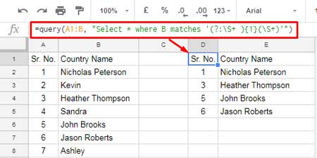
First, Middle, and Last Name:
See the result. If you want to filter only the names that contain the first name, middle name, and last name, replace {1} in the formula with {2}.
Query Formula to Filter Rows Based on the Number of Characters in a Column
This formula filters words that are two characters long:
=QUERY(A1:B, "SELECT * WHERE B MATCHES '..'")Increase the number of dots (periods) to match words with a greater number of characters.
Matches Regular Expression in Google Sheets Query to Match Texts Containing Vowels or Consonants
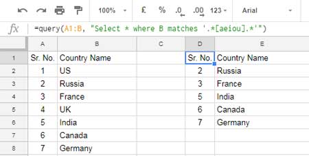
Formula 1:
=QUERY(A1:B, "SELECT * WHERE B MATCHES '.*[aeiou].*'")Formula 2:
=QUERY(A1:B, "SELECT * WHERE B MATCHES '.*[^aeiou].*'")I hope the above examples are sufficient to understand the use of the Matches regular expression match in Google Sheets Query.
Thanks for staying. Enjoy!


I have data for five to six months, and I want to compare sales from the 1st day to the 7th day of each month. Can I fetch data only for the first 7 days from all the data using the Query function in Google Sheets?
Yes, you can, but it depends on the layout.
Hi Prashanth,
Thank you for your detailed articles.
I am trying to create a Dashboard that can Filter through a Database and return a set of “Exercise Names” based on select Keywords, “Categories” and “Focus”. The Keywords are selected in Sheet1, under columns A,B, with up to 15 rows of the 2 Keywords to further filter the set of “Exercise Names”. In Sheet2, I have a list of “Exercise Names”, each with 5 columns of “Categories” (B,C,D,E,F is Category1, .. , Category5) and 15 Columns of “Focus” (G,H, .. , U is Focus1, Focus 2, .. , Focus 15).
How do I set up the Query so I can filter through Sheet2 (Columns B,C,D,E,F) to match the Keywords in Sheet1 (Column A), and also filter Sheet2(Columns G-U) to match the Keywords in Sheet1 (Column B), and display a specific set of Exercise Names?
Sorry, I’d be happy to provide my sheet info context helps!
Hi, David,
The problem seems solvable. It may require the use of functions like QUERY and TOCOL.
You may better share an example Sheet (URL) via the Reply below.
Please fill in only the necessary data and also your expected result.
Please guide us on how to remove all space and special characters in the Query function?
Hi, Monika,
Can I see a sample of your table?
You can post the Sheet URL via “Reply” to this comment.
Hey, Prashanth,
Thanks for these articles. They are the only ones that have helped me be somewhat closer to the answer to my query.
I have a column in Google sheets with data in the date-time format (E.g.: 2020-12-31 20:07:49). There are about 5600 such records spread across all times of the day. I want to calculate the number of calls received in a particular time slot. Say between 11:00 AM and 12:00 noon.
I’ve been struggling with timevalue, Countif, Countifs for about 3-4 days now, but am not able to figure it out. Will you be able to help? I’ll be greatly obliged.
Hi, Gurdeep,
See if this helps?
How to Count Events in Particular Timeslots in Google Sheets
Hi,
Can you tell me why the following query with Contains works but the one with Matches doesn’t? Eventually, I want to pipe more conditions in using
|but I need it to work first.Contains:
=QUERY(Raw!A2:P,"SELECT * WHERE K Contains ', 5/2/2020' ",0)Matches:
=QUERY(Raw!A2:P,"SELECT * WHERE K Matches '.*, 5/2/2020.*' ",0)Note:
The comment cutoff
<m>from both codes before the comma. So‘<m>, 5/2/2020’is the string I want to find.Hi, Jeff M,
From my test, both of your formulas work without any issues. Use correct apostrophes (single quotes) and double-quotes. Still problem? Then try the Matches formula as below.
=QUERY(Raw!A2:P,"SELECT * WHERE K matches '\<m\>\, 5\/2\/2020'",0)I’ve ‘escaped’ some characters in Matches using the backslash.
For multiple conditions in Matches use the Pipe.
Eg.:
=QUERY(Raw!A2:P,"SELECT * WHERE K matches '\<m\>\, 5\/2\/2020|\<m\>\, 5\/3\/2020'",0)Hi,
How can I match 3 words and a blank cell?
"SELECT Col1,Col2,Col3,Col5,Col7,Col8,Col9,Col11,Col24 WHERE Col5 = 1 AND Col11 Matches 'Partial Return|Returned|Re-attempt|'"Also, I want to compare a blank cell with ‘
Partial Return|Returned|Re-attempt'.Hi, Kiran,
Your formula already matches the said three strings and a blank cell in column 11.
'Partial Return|Returned|Re-attempt|'To remove blank in the output, remove the last pipe symbol as below.
'Partial Return|Returned|Re-attempt'Please rephrase your question, if you are asking something different.
Very informative. Is there anything that would allow me to query all items EXCEPT certain ones? For example, if I wanted a list that did not include ‘.*UK.*’ ?
Hi, Scott,
See if this helps?
CONTAINS Substring Match in Google Sheets Query for Partial Match