You can use the following formula to unstack multiple form responses in Google Sheets:
=LET(unq, UNIQUE(identifier_data), HSTACK(unq, BYROW(unq, LAMBDA(row, TOROW(FILTER(variable_data, TRANSPOSE(QUERY(TRANSPOSE(identifier_data),,9^9))=TRANSPOSE(QUERY(TRANSPOSE(row),,9^9))))))))Where:
identifier_datarepresents the user information part of the form responses.variable_datarepresents the response data part of the form responses.
This formula works by treating one section of the data as a unique user identifier and another section as variable data that will be transposed. Each section can have any number of columns.
Example: Unstacking Form Responses in Google Sheets
Sample Form Response
Consider the following form responses stored in the “Form responses 1” tab:
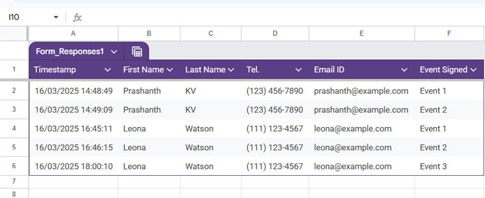
This is event registration data recorded in Google Sheets, where users who registered for multiple events submitted separate form responses instead of selecting multiple events in a single submission.
As shown, some users have submitted multiple responses.
Let’s now unstack multiple form responses using the formula.
Unstacking Multiple Form Responses
In the dataset, we first need to identify:
- Identifier Data → Columns B2:E6 (User information)
- Variable Data → Column F2:F6 (Event Signed)
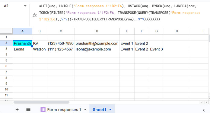
Now, enter the following formula in cell A2 of a new sheet:
=LET(unq, UNIQUE('Form responses 1'!B2:E6), HSTACK(unq, BYROW(unq, LAMBDA(row, TOROW(FILTER('Form responses 1'!F2:F6, TRANSPOSE(QUERY(TRANSPOSE('Form responses 1'!B2:E6),,9^9))=TRANSPOSE(QUERY(TRANSPOSE(row),,9^9))))))))This formula will unstack multiple form responses, ensuring that each user’s event registrations appear in a single row.
Note: I suggest entering the formula in A2 because you may want to manually arrange the headers in the first row.
Formula Breakdown
Step 1: Extract Unique User Information
UNIQUE('Form responses 1'!B2:E6)This returns the unique user identifier data from columns B to E, ensuring that each user appears only once.
Step 2: Filter and Transpose Event Data
BYROW(unq, LAMBDA(row, TOROW(FILTER('Form responses 1'!F2:F6,
TRANSPOSE(QUERY(TRANSPOSE('Form responses 1'!B2:E6),,9^9))=TRANSPOSE(QUERY(TRANSPOSE(row),,9^9))
))))TRANSPOSE(QUERY(TRANSPOSE(…)))– Combines multiple identifier columns into a single-column reference (for comparison).TRANSPOSE(QUERY(TRANSPOSE(row),,9^9)))– Converts the current row of unique identifier columns into a single-column reference (to match users).FILTER(…)– Extracts the event data for each user by matching their unique identifier data.BYROW(…)– Iterates through each unique user and arranges their event responses into a single row.TOROW(…)– Converts the filtered results into a horizontal format.
Step 3: Stack the Data
HSTACK(unq, ...)This horizontally stacks the unique user identifier data (unq) with the structured event data returned by BYROW.
The formula effectively unstacks multiple form responses into a structured format, ensuring each user’s event registrations appear in a single row.
Unstacking Multiple Form Responses with Dynamic Ranges
To ensure future form responses are also unstacked dynamically, replace fixed ranges with open ranges:
=LET(unq, UNIQUE('Form responses 1'!B2:E), HSTACK(unq, BYROW(unq, LAMBDA(row, TOROW(FILTER('Form responses 1'!F2:F, TRANSPOSE(QUERY(TRANSPOSE('Form responses 1'!B2:E),,9^9))=TRANSPOSE(QUERY(TRANSPOSE(row),,9^9))))))))This ensures new responses are automatically included.
Using Structured Table References
Alternatively, you can use structured table references for better readability:
=LET(unq, UNIQUE(Form_Responses1[First Name]:Form_Responses1[Email ID]), HSTACK(unq, BYROW(unq, LAMBDA(row, TOROW(FILTER(Form_Responses1[Event Signed], TRANSPOSE(QUERY(TRANSPOSE(Form_Responses1[First Name]:Form_Responses1[Email ID]),,9^9))=TRANSPOSE(QUERY(TRANSPOSE(row),,9^9))))))))Why Use Structured Table References?
- Easier to read and manage
- Auto-adjusts when new data is added
- Improves formula maintainability
If you’re new to structured table references, check out this guide: Structured Table References in Google Sheets.
Conclusion
The unstack multiple form responses formula in Google Sheets allows you to efficiently reorganize form submissions, grouping related responses by unique users. Whether using standard ranges or structured references, this method ensures a clean, structured dataset for further analysis.


