You don’t need any plugins or Apps Script to unstack data in Google Sheets. All you need is my custom array formula.
Understanding Unstacking Data
Before we dive into unstacking data into corresponding groups in Google Sheets, let’s clarify what “unstacking data” means.
Stacked Data, also known as long-format data, has key characteristics that set it apart from unstacked (wide-format) data:
- In stacked data, each row generally shows one record or entry related to a specific detail. For example, in a dataset tracking sales, each row might represent an individual sale.
- Each row often includes an item, its category, and quantity. The next row may represent a different or the same item, possibly under the same or a different category, with its corresponding quantity.
Unstacking transforms stacked data into a format where categories or groups are represented as separate columns, allowing for easier analysis and visualization.
For instance, unstacking can organize items and their quantities under each respective category in separate columns, grouping data more visibly by category.
Side note: Long-format (stacked) data is especially useful for statistical analysis in Google Sheets. You can use functions like QUERY or the Pivot Table tool to summarize the data, and also apply lookup functions more efficiently.
Unstacking Two-Column Stacked Data in Google Sheets
Consider a sample dataset with country names in column A and their assigned groups in a football event in column B. This is stacked data since each row represents a single team.
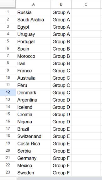
When unstacking, there will be a key column. In this case, column B contains the groups assigned to each country.
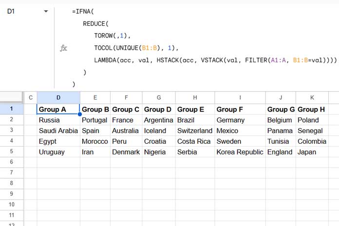
You can use the following formula in cell D1 to unstack the data in columns A and B:
=IFNA(
   REDUCE(
      TOROW(,1),
      TOCOL(UNIQUE(B1:B), 1),
      LAMBDA(acc, val, HSTACK(acc, VSTACK(val, FILTER(A1:A, B1:B=val))))
   )
)
In this formula, replace B1:B with the key (category) column and A1:A with the other column.
Formula Breakdown
This formula is simple to implement, but it can be somewhat complex to understand, as it uses a custom LAMBDA function within the REDUCE function. Here’s a step-by-step explanation of the formula: LAMBDA(acc, val, HSTACK(acc, VSTACK(val, FILTER(A1:A, B1:B=val)))).
Understanding the REDUCE Function:
The REDUCE function takes an initial value (an empty array specified as TOROW(,1)) and applies the LAMBDA function to each value in the unique array: TOCOL(UNIQUE(B1:B), 1).
Key Elements of the LAMBDA Function:
FILTER(A1, B1=val)– This part filters the country names inA1:Awhere the group inB1:Bmatchesval. Here,valrefers to a unique group name from column B. For instance, ifvalis “Group A,” the formula will return:Russia
Saudi Arabia
Egypt
UruguayVSTACK(val, FILTER(A1, B1=val))– This vertically stacks theval(e.g., “Group A”) with the filtered data, resulting in:Group A
Russia
Saudi Arabia
Egypt
UruguayHSTACK(acc, VSTACK(val, FILTER(A1, B1=val)))– The HSTACK function horizontally appends the accumulated result (acc) with the output from the previous step. In the LAMBDA function,accrefers to the accumulated data, andvalrepresents each unique category in column B:LAMBDA(acc, val, HSTACK(acc, VSTACK(val, FILTER(A1:A, B1:B=val))))
As a result, you obtain the unstacked data.
Unstacking Three-Column Stacked Data in Google Sheets
In the next example, suppose we have item names in column A, their categories in column B, and quantities in column C.
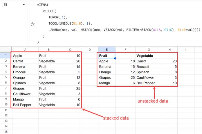
To unstack the data based on the category in column B, we’ll modify the filter slightly.
Previously, the formula was:
FILTER(A1:A, B1:B=val)Now, we want to include both A1:A and C1:C, so the filter becomes:
FILTER(HSTACK(A1:A, C1:C), B1:B=val)The updated formula will be:
=IFNA(
   REDUCE(
      TOROW(,1),
      TOCOL(UNIQUE(B1:B), 1),
      LAMBDA(acc, val, HSTACK(acc, VSTACK(val, FILTER(HSTACK(A1:A, C1:C), B1:B=val))))
   )
)
Conclusion
That’s all about how to unstack data in Google Sheets. This process allows you to organize your data into a more usable format for analysis.
Resources
- How to Stack Data in Google Sheets: Tips and Tricks
- Unstack Multiple Form Responses in Google Sheets
- A Simple Formula to Unpivot a Dataset in Google Sheets
- Unpivot Excel Data Fast: Power Query & Dynamic Array Formula
- Split Your Google Sheet Data into Category-Specific Tables
- Dynamic Formula: Split a Table into Multiple Tables in Google Sheets


Hi Prashanth!
Thank you for this wonderful resource!
I have some stacked data that is in 5 columns. Column headings are as follows:
Survey | Language | ID | Question | Value
Is there an expanded version of this formula that would work for me?
Many thanks!
Hi, Nate,
I don’t have a formula for that. I have a distantly related tutorial titled “How to Aggregate Strings Using Query in Google Sheets” which I have linked in one of my earlier replies.
Also, please see this tutorial.
Formula to Combine Duplicate Rows in Google Sheets [No-Addon]
See if that helps?
Best,
Hello. Thank you for your great article. I have tried the solution for a Google Sheet I am working on however it is not producing the results we hoped for. I have a list of attendees for different events. The columns are First Name, Last Name, Email, and Event.
The first three columns (Name, Last Name, Email) will contain the same information when someone signed up for a unique event. The data looks like this.
first name A | last name A | email A | Event Name 1
first name A | last name A | email A | Event Name 2
first name B | last name B | email A | Event Name 1
etc.
What we would like to do is have a single row with:
First Name, Last Name, Email, Event 1, Event, 2, etc. from our current stacked data.
First Name A | Last Name A | email A | Event Name 1 | Event Name 2
First Name B | Last Name B | email B | Event Name 1
Is this possible with Google Sheets?
Thank you in advance for your time.
Hi, Joe,
Welcome to Info Inspired!
The tutorial above is not the one that you may want to follow. Here is the proper one – How to Aggregate Strings Using Query in Google Sheets.
The tutorial contains the basic but only deals with two columns of data. Since you have more columns I have customized the formula for you. Here is that.
=ArrayFormula(query(query({A2:D,if(len(A2:A),row(A2:A)-match(A2:A&B2:B,A2:A&B2:B,0),)},"Select Col1,Col2,Col3, max(Col4) where Col1 is not null group by Col1,Col2,Col3 Pivot Col5"),"Select * offset 1",0))Make sure that you have sorted your data.
I am considering the data range A2:D (I am normally leaving the first row as it may contain field labels). So adjust your data accordingly.
Please do check the tutorial (link shared above) to understand this formula.
Best,