The Google Sheets SORT function is a formula that can be used to sort data in a spreadsheet. It is an alternative to the SORT menu command in the application. Unlike the menu command, the formula returns the sorted values in a new range.
SORT Function vs. SORT Menu in Google Sheets
There are a few noticeable advantages of using the SORT function over traditional menu-based sorting in Google Sheets.
Pros
- If you use the Data > Sort sheet or Sort range menu commands, you may need to sort the data again if you update the range. However, the SORT function will update instantly without user interference, provided the edited value is within the sort range.
- The question of undo sorting does not arise when you use a formula for sorting a range or sheet because it does not alter the source range.
- It is easy to sort other formula results using a SORT wrapper around them.
- Both the menu command and the function are for sorting vertical data. However, when using the function, we can additionally use the TRANSPOSE function to change the data orientation and make horizontal sorting possible.
- The LOOKUP function is one of the most popular functions in Google Sheets. It requires a sorted range to work. If your data range is unsorted and you do not want to disturb that, you can use the Google Sheets SORT function within the LOOKUP function to create a virtual sorted data range.
I have included some additional tips in this SORT function tutorial with the LOOKUP function in mind.
Also, there are plenty of resources related to sorting data on this blog. I have included some of the relevant tutorial links at the bottom of this tutorial.
Cons
What are the disadvantages of the SORT function over the menu commands?
The SORT function has a few disadvantages over the menu commands. First, we cannot directly edit the sorted range. Editing the sorted range will break the formula.
Second, the Data menu Create a filter menu command has a sort feature that allows us to sort a cell range by fill color. This is not possible when using the formula.
SORT Function in Google Sheets: Syntax and Arguments
Syntax:
SORT(range, sort_column, is_ascending, [sort_column2, …], [is_ascending2, …])Arguments:
range: The range (data) to be sorted. It can contain more than one column.
sort_column: The index (column number) of the column in range or a range outside. The function will sort the range containing the values in the index column. It must be a single column with the same number of rows as the range.
I will share more about sorting based on the sort_column outside range in the example section below.
is_ascending: TRUE or FALSE indicating whether to sort sort_column in ascending (A-Z) or descending order (Z-A). We can replace TRUE with 1 and FALSE with 0 (zero), where 1 means ascending order and 0 means descending order.
sort_column2, is_ascending2 …: Optional arguments to specify additional sort_columns and sort order (is_ascending) flags beyond the first, in order of precedence.
Now, let’s see how to use the Google Sheets SORT function.
Usage Examples of Google Sheets SORT Function
I assume you have already gone through the syntax section above and also the advantages and disadvantages of using the SORT function just above it.
Without examples, you may not be able to understand the function fully. Here are the simplest examples to understand how to use the SORT function in Google Sheets with ease.
Basic Example
When you have a column with text, numbers, dates, or mixed-type data, the Google Sheets SORT function will sort the column as follows:
- Numeric and date values are sorted numerically.
- Text values are sorted alphabetically.
- Logical values are sorted by their Boolean value. In ascending order, FALSE comes before TRUE, and in descending order, TRUE comes before FALSE.
- Empty cells are segregated at the end of the range.
The order of the values in a mixed-type data column will be:
- Ascending order (A-Z): Numeric values and dates > text > logical values > empty cells.
- Descending order (Z-A): Logical values > text > numbers and dates > empty cells.
To illustrate the above points, let’s sort a mixed data type column.
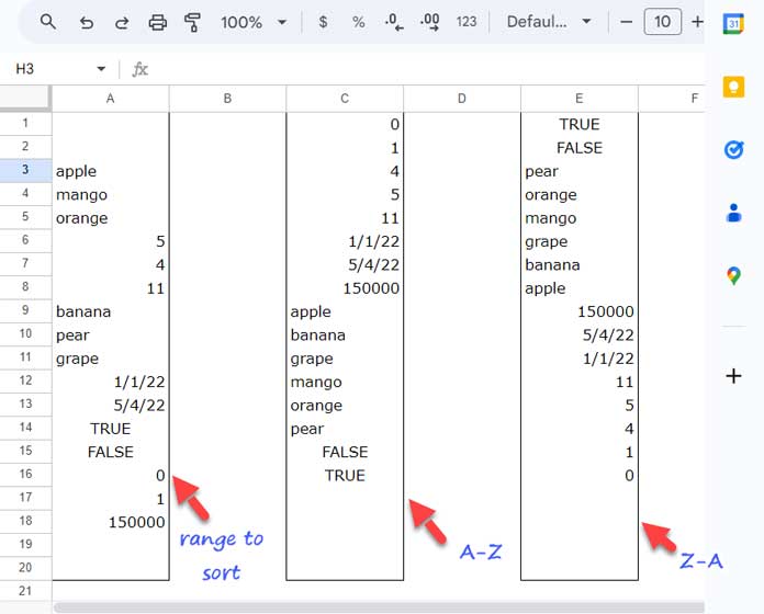
The following SORT formula in cell C2 sorts the mixed data type column range A1:A20 in ascending order.
=SORT(A1:A20,1,TRUE)range: A1:A20
sort_column: 1
is_ascending: TRUE
Here is the formula in cell E2 which sorts the same range in descending order.
=SORT(A1:A20,1,FALSE)range: A1:A20
sort_column: 1
is_ascending: FALSE
Single Sort Column
In the above example, we have used a single sort column. There is only one column to sort, so the question of sorting two sort columns does not arise.
Here is one more example with a single sort column in the Google Sheets SORT function. This time, we have two columns in the range to sort.
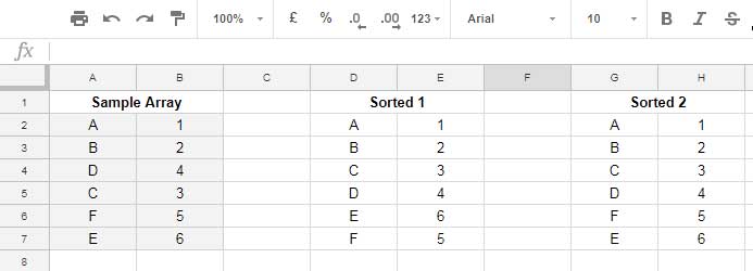
Formula 1 (in cell D2):
=SORT(A2:B7,1,TRUE)In this formula, the range is A2:B7 and sort_column is column 1. The formula sorts the array/range based on the first column in ascending order.
Formula 2 (in cell G2):
=SORT(A2:B7,2,TRUE)This formula is the same as formula 1 above but with one difference. The difference is that the sort_column argument is set to 2. This means that the formula will sort the array A2:B7 based on column 2.
Here, too, I have sorted the range in ascending order. You can just replace TRUE with FALSE to sort the range in descending order.
Multiple Sort Columns
We often need to use multiple sort columns when using the SORT function in Google Sheets.
For example, to find the latest entry in each group, you might first sort the group column in ascending order and a date column in descending order.
Here is an example of how to do this.
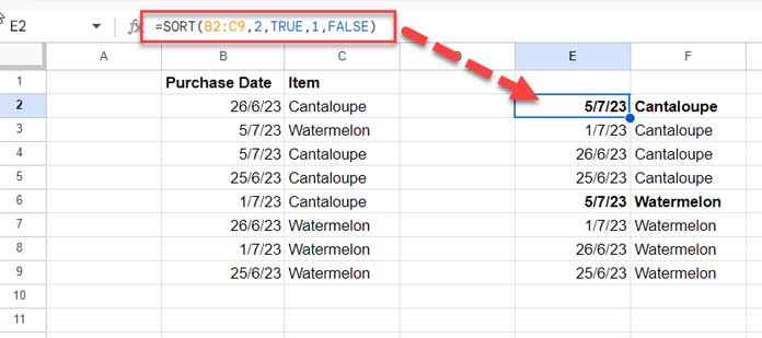
=SORT(B2:C9,2,TRUE,1,FALSE)range: B2:C9
sort_column: 2
is_ascending: TRUE
sort_column: 1
is_ascending: FALSE
The formula first sorts the fruit names (Item) in ascending order and then the date of purchase (Purchase Date) in descending order. This means that the latest purchased items will appear at the top of each group.
As per the above example, the latest purchase of Cantaloupe and Watermelon is on 05th July 2023.
Tip
We can use the SORTN function to extract these two items.
=SORTN(SORT(B2:C9,2,TRUE,1,FALSE),9^9,2,2,1)Can the column index in the SORT function in Google Sheets be replaced with a range reference?
The answer is yes. To clarify, I am replacing the sort_column index numbers 2 and 1 with the corresponding ranges below.
=SORT(B2:C9,C2:C9,TRUE,B2:B9,FALSE)range: B2:C9
sort_column: C2:C9
is_ascending: TRUE
sort_column: B2:B9
is_ascending: FALSE
Google Sheets SORT Function and Sorting Based on an Outside Range
In the previous SORT function examples, the sort_column was from within the sort range.
In the following example, I want to use the Google Sheets SORT function to sort the range B2:C8 based on the numbers (ranks) in E2:E8, which is a distant range.
Here, the sort_column is an outside range, so we must use a range reference instead of a column index in the sort.
=sort(B2:C8,E2:E8,1)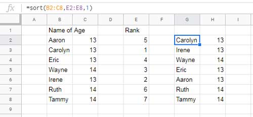
Google Sheets Sort Function: Tips and Tricks
I think the above SORT function usage examples are enough for one to learn this function. Here are some additional tips and tricks related to the Google Sheets SORT function.
Horizontal Range
At the beginning of this tutorial, I shared one of the advantages of the Google Sheets SORT function over the menu command: it can sort horizontal data sets.
The function is built-in to sort vertical data sets, as shown in the above examples. However, if you want to use it in a horizontal data set, you can use the TRANSPOSE function with it.
I have already explained this topic in one of my other tutorials. Please refer to that for more information: How to Sort Horizontally in Google Sheets.
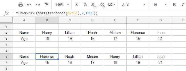
Alternatively, you can also refer to the screenshot below. It shows how to sort horizontal data in Google Sheets using the TRANSPOSE and SORT functions.
Example:
You May Also Like: Row-Wise Sorting in a 2-D Array in Google Sheets.
Sort Without Specifying Sort Index Column
You might have seen the below usage of the SORT function, which only contains the range.
=SORT(A2:B5)Such formulas are used to sort the data by its first column in ascending order.
FILTER Function with SORT Function: Combination Use to Remove Blank Cells
The FILTER function in Google Sheets returns a filtered version of the source range. This means that we can use it to filter out values in a range before sorting.
Here, we will use it to filter out the blank rows in the sorted result.
The SORT function moves the blank cells in the sort column to the bottom of the range. We can remove such blank cells using the FILTER function. Here is an example of this.
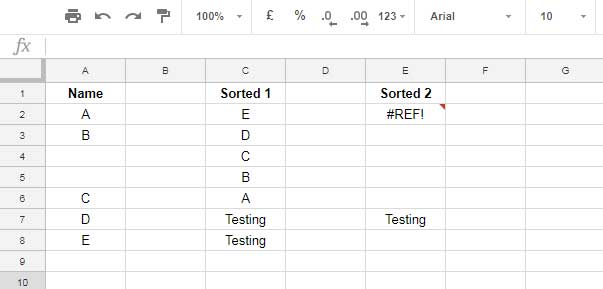
In cell range A2:A8, we have five letters. We want to sort them in cell E2 and get the result limited to E2:E6.
However, the following formula in cell E2 returns a #REF! error because it cannot expand due to the value in cell E7:
=SORT(A2:A8,1,FALSE)The solution is to filter out the blank cells in the sorted data so that it can fit into E2:E6. Here is the formula:
=FILTER(SORT(A2:A8,1,FALSE),SORT(A2:A8,1,FALSE)<>"")The above formula is not resource-friendly because it executes the SORT function twice. We can solve that using the LET function as follows:
=LET(srt,SORT(A2:A8,1,FALSE),FILTER(srt,srt<>""))SORT Function to Create a Virtual Sorted Range in LOOKUP Function in Google Sheets
The LOOKUP function looks up a value (search key) in a sorted row or column and returns the corresponding value from another range. If the range is not sorted, the LOOKUP function will not work correctly.
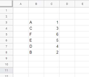
Here is how to use the Google Sheets SORT function within the LOOKUP function to sort the data and look up a value.
=LOOKUP("F",SORT(B3:C8))Similar: How to Use LOOKUP Function in an Unsorted Array in Google Sheets.
Conclusion
N/A! is the most common error that you may encounter when using the Google Sheets SORT function. It can be due to many reasons, but here are the most prominent ones:
SORT expects all arguments after position 1 to be in pairs: This means that you haven’t specified the is_sorted Boolean value.
SORT has mismatched range sizes: This means that the range that you are sorting and the range that you are using for the sort column are not the same size.
A wrong number of arguments to SORT: This means that you are not providing the correct number of arguments to the SORT function. This is most common when you use a formula within the SORT function, such as the FILTER function, which returns a blank if there are no matching values.
Resources:


